Array Code in C++

As we have learned in Matrix Operations, Cache Optimization, and SIMD (Vector Processing), fast code calls for regular access to compact data. Not all data structures offer fast runtime. For writing fast code, arrays are the simplest and most commonly used data structure. We will discuss how to use arrays to achieve high speed.

Python Is Slow

When using Python for number-crunching, the fact of its slowness needs to be kept in mind always. Handling the slowness is the key to make Python run as fast as C.

Here we consider a boundary value problem of the Laplace equation for temperature distribution in a \(1\times1\) square area.

\[\begin{split}& \frac{\partial^2 u}{\partial x^2} + \frac{\partial^2 u}{\partial y^2} = 0 \quad (0<x<1; 0<y<1) \\ &\left\{\begin{array}{lll} u(0,y) = 0, & u(1,y) = \sin(\pi y) & \rule{4ex}{0pt} (0 \le y \le 1) \\ u(x,0) = 0, & u(x,1) = 0 & \rule{4ex}{0pt} (0 \le x \le 1) \end{array}\right.\end{split}\]

Laplace Equation in Python

To solve it numerically, we choose the finite-difference method. The finite-difference method needs a grid to discretize the spatial domain. The simplest spatial discretization is the homogeneous Cartesian grid. Let’s make a \(51\times51\) Cartesian grid. The Python code is:

import numpy as np

def make_grid():
    # Number of the grid points.
    nx = 51
    # Produce the x coordinates.
    x = np.linspace(0, 1, nx)
    # Create the two arrays for x and y coordinates of the grid.
    gx, gy = np.meshgrid(x, x)
    # Create the field and zero-initialize it.
    u = np.zeros_like(gx)
    # Set the boundary condition.
    u[0,:] = 0
    u[-1,:] = 1 * np.sin(np.linspace(0,np.pi,nx))
    u[:,0] = 0
    u[:,-1] = 0
    # Return all values.
    return nx, x, u

nx, x, uoriginal = make_grid()

The full code is in 01_grid.py. Plot the grid using matplotlib:

A Cartesian grid of \(51\times51\) grid points.

After the grid is defined, we derive the finite-differencing formula. Use the Taylor series expansion to obtain the difference equation:

\[\begin{split}& \frac{u(x_{i+1}, y_j) - 2u(x_i, y_j) + u(x_{i-1}, y_j)}{(\Delta x)^2} \\ &\quad + \frac{u(x_i, y_{j+1}) - 2u(x_i, y_j) + u(x_i, y_{j+1})}{(\Delta y)^2} = 0\end{split}\]

Note \(\Delta x = \Delta y\). The difference equation is rewritten as

\[u(x_i, y_j) = \frac{u(x_{i+1}, y_j) + u(x_{i-1}, y_j) + u(x_i, y_{j+1}) + u(x_i, y_{j-1})}{4}\]

Apply the point-Jacobi method to write a formula to iteratively solve the difference equation:

\[u^{n+1}(x_i, y_i) = \frac{u^n(x_{i+1}, y_j) + u^n(x_{i-1}, y_j) + u^n(x_i, y_{j+1}) + u^n(x_i, y_{j-1})}{4}\]

where \(u^n\) is the solution at the \(n\)-th iteration.

Using the above formula, we are ready to implement the solver in Python. The code is short and straight-forward:

def solve_python_loop():
    u = uoriginal.copy()  # Input from outer scope
    un = u.copy()  # Create the buffer for the next time step
    converged = False
    step = 0
    # Outer loop.
    while not converged:
        step += 1
        # Inner loops. One for x and the other for y.
        for it in range(1, nx-1):
            for jt in range(1, nx-1):
                un[it,jt] = (u[it+1,jt] + u[it-1,jt] + u[it,jt+1] + u[it,jt-1]) / 4
        norm = np.abs(un-u).max()
        u[...] = un[...]
        converged = True if norm < 1.e-5 else False
    return u, step, norm

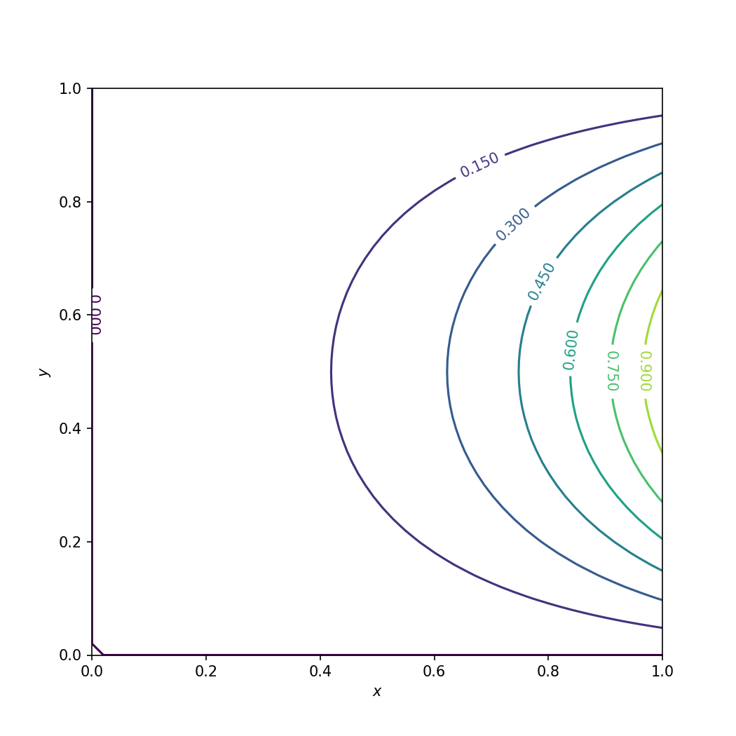
The full code is in 01_solve_python_loop.py. The solution can be plotted using matplotlib:

Numerical solution of the Laplace equation in Python.

The solution takes quite a while (4.797 seconds) to converge using 2097 iterations:

>>> with Timer():
>>>    u, step, norm = solve_python_loop()
>>> print(step)
Wall time: 4.79688 s
2097

Analytical Solution

Is the calculation correct? It is the first question to ask for any numerical application.

We may compare the numerical solution to the analytical solution. Recall the PDE and its boundary conditions:

\[\begin{split}& \frac{\partial^2 u}{\partial x^2} + \frac{\partial^2 u}{\partial y^2} = 0 \quad (0<x<1; 0<y<1) \\ &\left\{\begin{array}{lll} u(0,y) = 0, & u(1,y) = \sin(\pi y) & \rule{4ex}{0pt} (0 \le y \le 1) \\ u(x,0) = 0, & u(x,1) = 0 & \rule{4ex}{0pt} (0 \le x \le 1) \end{array}\right.\end{split}\]

Use separation of variable. Assume the solution \(u(x,y) = \phi(x)\psi(y)\).

\[\begin{split}& \frac{\partial^2 u}{\partial x^2} + \frac{\partial^2 u}{\partial y^2} = 0 \quad \Rightarrow \quad \phi''\psi + \phi\psi'' = 0 \\ & \Rightarrow \quad \frac{\phi''}{\phi} = -\frac{\psi''}{\psi} = \lambda\end{split}\]

\[\begin{split}\left\{\begin{array}{ll} \phi'' - \lambda\phi = 0, & \phi(0) = 0 \\ \psi'' + \lambda\psi = 0, & \psi(0) = 0, \, \psi(1) = 0 \end{array}\right.\end{split}\]

\(\lambda\) is the eigenvalue. The general solution of the ODE of \(\psi\) can be obtained as

\[\psi(y) = c\cos(\kappa y) + d\sin(\kappa y), \quad \kappa^2 = \lambda\]

Substitute the boundary conditions to the general solution

\[\begin{split}& \psi(0) = c = 0 \, \Rightarrow \, c = 0 \\ & \psi(1) = d\sin(\kappa) = 0 \, \Rightarrow \, \kappa = n\pi, \, n = 1, 2, 3, \ldots \\ & \psi(y) = \sum_{n=1}^{\infty} \psi_n(y), \; \mbox{where} \; \psi_n(y) = d_n\sin(n\pi y) \\ & \Rightarrow \psi(y) = \sum_{n=1}^{\infty} d_n \sin(n\pi y)\end{split}\]

Substitute the eigenvalue \(\lambda\) into the ODE of \(\phi\)

\[\phi'' - (n\pi)^2\phi = 0\]

The general solution is

\[\phi_n(x) = a_n\cosh(\kappa x) + b_n\sinh(\kappa x)\]

Apply the boundary condition \(\phi_n(0) = a_n = 0\) and obtain \(\phi_n(x) = b_n\sinh(\kappa x)\).

The solution \(u(x, y)\) can now be written as

\[u(x,y) = \sum_{n=1}^{\infty}\phi_n(x)\psi_n(y) = \sum_{n=1}^{\infty} \alpha_n \sinh(n\pi x)\sin(n\pi y)\]

where \(\alpha_n = b_nd_n\). Apply the last boundary condition

\[u(1,y) = \sin(\pi y) = \sum_{n=1}^{\infty}\alpha_n\sinh(n\pi)\sin(n\pi)\]

to obtain that \(\alpha_1 = \sinh^{-1}(\pi)\) and \(\alpha_n = 0 \; \forall \; n > 1\). The solution of \(u\) is then determined:

\[u(x, y) = \frac{\sinh(\pi x)}{\sinh(\pi)} \sin(\pi y)\]

def solve_analytical():
    u = np.empty((len(x), len(x)), dtype='float64')
    for ix, cx in enumerate(x):
        u[ix, :] = np.sinh(np.pi*cx) / np.sinh(np.pi) * np.sin(np.pi*x)
    return u

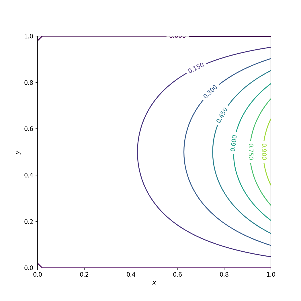
The full code is in 01_solve_analytical.py. The solution is plotted:

Analytical solution of the Laplace equation.

Say \(u_a\) is the analytical solution. The numerical solution is compared against the analytical solution, and the result \(|u-u_a|_{\infty} < 0.005\) is good enough.

>>> uanalytical = solve_analytical()
>>> # Calculate the L inf norm.
>>> print("Linf of difference is %f" % np.abs(u - uanalytical).max())
Linf of difference is 0.004962

Array-Based Code with Numpy

To speed up the slow Python loops, numpy is usually a solution. Numpy implements fast calculations in C. By using numpy, the intensive calculation is delegated to C.

def solve_array():
    u = uoriginal.copy()  # Input from outer scope
    un = u.copy()  # Create the buffer for the next time step
    converged = False
    step = 0
    while not converged:
        step += 1
        un[1:nx-1,1:nx-1] = (u[2:nx,1:nx-1] + u[0:nx-2,1:nx-1] +
                             u[1:nx-1,2:nx] + u[1:nx-1,0:nx-2]) / 4
        norm = np.abs(un-u).max()
        u[...] = un[...]
        converged = True if norm < 1.e-5 else False
    return u, step, norm

The full code is in 02_solve_array.py. The solution is verified to be the same as that with naive Python loops and then plotted:

Numerical solution of the Laplace equation using numpy.

The speed is much better: less than 0.1 second. Compared to that of the naive Python loops, the speed up is more than 50x (to be exact, 87x):

>>> # Run the Python solver
>>> with Timer():
>>>     u, step, norm = solve_array()
Wall time: 0.0552309 s

Nested Loop in C++

While numpy does speed up the naive Python loops, it has two drawbacks:

1. It is still not optimal speed.

2. The code is not easy to read, compared to the element-wise code in the loop version. Nested loop reads more straight-forward for our point-Jacobi method.

Here we will see how much faster it can get to move the code from numpy to C++. To simplify the implementation, I use an array library from modmesh. It helps to organize the code and achieve faster runtime.

Except the parentheses, the C++ version looks almost the same as the Python version.

std::tuple<modmesh::SimpleArray<double>, size_t, double>
solve1(modmesh::SimpleArray<double> u)
{
    const size_t nx = u.shape(0);
    modmesh::SimpleArray<double> un = u;
    bool converged = false;
    size_t step = 0;
    double norm;
    while (!converged)
    {
        norm = 0.0;
        ++step;
        for (size_t it=1; it<nx-1; ++it)
        {
            for (size_t jt=1; jt<nx-1; ++jt)
            {
                un(it,jt) = (u(it+1,jt) + u(it-1,jt) + u(it,jt+1) + u(it,jt-1)) / 4;
                double const v = std::abs(un(it,jt) - u(it,jt));
                if (v > norm)
                {
                    norm = v;
                }
            }
        }
        // additional loop slows down: norm = calc_norm_amax(u, un);
        if (norm < 1.e-5) { converged = true; }
        u = un;
    }
    return std::make_tuple(u, step, norm);
}

// Expose the C++ helper to Python
PYBIND11_MODULE(solve_cpp, m)
{
    // Boilerplate for using the SimpleArray with Python
    {
        modmesh::python::import_numpy();
        modmesh::python::wrap_ConcreteBuffer(m);
        modmesh::python::wrap_SimpleArray(m);
    }
    m.def
    (
        "solve_cpp"
      , [](pybind11::array_t<double> & uin)
        {
            auto ret = solve1(modmesh::python::makeSimpleArray(uin));
            return std::make_tuple(
                modmesh::python::to_ndarray(std::get<0>(ret)),
                std::get<1>(ret),
                std::get<2>(ret));
        }
    );
}

The full C++ code is in solve_cpp.cpp. The Python driver code for the C++ kernel is in 03_solve_cpp.py. We verify the C++ code is to verify the solution is the same as before. It is plotted:

Numerical solution of the Laplace equation using C++.

Then we time the C++ version:

>>> with Timer():
>>>     u, step, norm = solve_cpp.solve_cpp(uoriginal)
Wall time: 0.0251369 s

It is twice as fast as the numpy version (0.0552309 seconds).

Overall Comparison

Now make a comparison for the three different implementations.

Runtime Performance

By putting all timing data in a table, it is clear how much the C++ version wins:

Runtime with Python loop, Numpy array, and C++ loop.

Code	Time (s)	Speedup
Python nested loop	4.797	1 (baseline)	n/a
Numpy array	0.055	87.22	1 (baseline)
C++ nested loop	0.025	191.88	2.2

Readability and/or Maintainability

To compare the easy-of-reading among the three versions, we list the three different computing kernels side by side:

Element-wise kernel using pure Python (full case in Laplace Equation in Python).

for it in range(1, nx-1):
    for jt in range(1, nx-1):
        un[it,jt] = (u[it+1,jt] + u[it-1,jt] + u[it,jt+1] + u[it,jt-1]) / 4

Element-wise kernel using numpy (full case in Array-Based Code with Numpy).

un[1:nx-1,1:nx-1] = (u[2:nx,1:nx-1] + u[0:nx-2,1:nx-1] +
                     u[1:nx-1,2:nx] + u[1:nx-1,0:nx-2]) / 4

Element-wise kernel using C++ (full case in Nested Loop in C++).

for (size_t it=1; it<nx-1; ++it)
{
    for (size_t jt=1; jt<nx-1; ++jt)
    {
        un(it,jt) = (u(it+1,jt) + u(it-1,jt) + u(it,jt+1) + u(it,jt-1)) / 4;
    }
}

Overhead in Data Preparation

Numerical calculation takes time. Intuitively, developers spend time on optimizing the number-crunching code. However, for a useful application, the house-keeping code for preparing the calculation data and post-processing the results is equally important.

In our previous example of solving the Laplace equation, all the conditions are hard-coded. It’s OK for the teaching purpose, but not useful to those who don’t know so much about the math and numerical. This time, I will use an example of polynomial curve fitting for variable-size data groups to show how the house-keeping code affects performance.

Least-Square Regression

The problem is to find an \(n\)-th order algebraic polynomial function

\[p_n(x) = \sum_{i=0}^n a_ix^i\]

such that there is \(\min(f(\mathbf{a}))\), where the \(L_2\) norm is

\[f(\mathbf{a}) = \sum_{k=1}^m\left(p_n(x_k) - y_k\right)^2\]

for the point cloud \((x_k, y_k), \; k = 1, 2, \ldots, m\). For the function \(f\) to have global minimal, there must exist a vector \(\mathbf{a}\) such that \(\nabla f = 0\). Take the partial derivative with respected to each of the polynomial coefficients \(a_0, a_1, \ldots, a_n\)

\[\begin{split}\frac{\partial f}{\partial a_i} & = \frac{\partial}{\partial a_i} \left[ \sum_{k=1}^m \left( \sum_{j=0}^n a_jx_k^j - y_k \right) \right]^2 \\ & = 2 \sum_{k=1}^m x_k^i \left( \sum_{j=0}^n a_jx_k^j - y_k \right) \\ & = 2 \sum_{k=1}^m \left( \sum_{j=0}^n a_jx_k^{i+j} - x_k^iy_k \right) , \; i = 0, 1, \ldots, n\end{split}\]

Because \(\frac{\partial f}{\partial a_i} = 0\), we obtain

\[\sum_{j=0}^n a_j \sum_{k=1}^m x_k^{i+j} = \sum_{k=1}^m x_k^iy_k\]

The equations may be written in the matrix-vector form

\[\mathrm{M}\mathbf{a} = \mathbf{b}\]

The system

\[\begin{split}\mathrm{M} = \left(\begin{array}{ccccc} m & \sum_{k=1}^m x_k^1 & \sum_{k=1}^m x_k^2 & \cdots & \sum_{k=1}^m x_k^n \\ \sum_{k=1}^m x_k^1 & \sum_{k=1}^m x_k^2 & \sum_{k=1}^m x_k^2 & \cdots & \sum_{k=1}^m x_k^{1+n} \\ \sum_{k=1}^m x_k^2 & \sum_{k=1}^m x_k^3 & \sum_{k=1}^m x_k^4 & \cdots & \sum_{k=1}^m x_k^{2+n} \\ \vdots & \vdots & \vdots & \ddots & \vdots \\ \sum_{k=1}^m x_k^n & \sum_{k=1}^m x_k^{n+1} & \sum_{k=1}^m x_k^{n+2} & \cdots & \sum_{k=1}^m x_k^{2n} \end{array}\right)\end{split}\]

The vector for the polynomial coefficients and the right-hand side vector are

\[\begin{split}\mathbf{a} = \left(\begin{array}{c} a_0 \\ a_1 \\ a_2 \\ \vdots \\ a_n \end{array}\right), \; \mathbf{b} = \left(\begin{array}{c} \sum_{k=1}^m y_k \\ \sum_{k=1}^m x_ky_k \\ \sum_{k=1}^m x_k^2y_k \\ \vdots \\ \sum_{k=1}^m x_k^ny_k \end{array}\right)\end{split}\]

The full example code is in data_prep.cpp. The Python driver is in 04_fit_poly.py.

This is the helper function calculating the coefficients of one fitted polynomial by using the least square regression:

C++ function for fitting a single polynomial function.

/**
 * This function calculates the least-square regression of a point cloud to a
 * polynomial function of a given order.
 */
modmesh::SimpleArray<double> fit_poly
(
    modmesh::SimpleArray<double> const & xarr
  , modmesh::SimpleArray<double> const & yarr
  , size_t start
  , size_t stop
  , size_t order
)
{
    if (xarr.size() != yarr.size())
    {
        throw std::runtime_error("xarr and yarr size mismatch");
    }

    // The rank of the linear map is (order+1).
    modmesh::SimpleArray<double> matrix(std::vector<size_t>{order+1, order+1});

    // Use the x coordinates to build the linear map for least-square
    // regression.
    for (size_t it=0; it<order+1; ++it)
    {
        for (size_t jt=0; jt<order+1; ++jt)
        {
            double & val = matrix(it, jt);
            val = 0;
            for (size_t kt=start; kt<stop; ++kt)
            {
                val += pow(xarr[kt], it+jt);
            }
        }
    }

    // Use the x and y coordinates to build the vector in the right-hand side
    // of the linear system.
    modmesh::SimpleArray<double> rhs(std::vector<size_t>{order+1});
    for (size_t jt=0; jt<order+1; ++jt)
    {
        rhs[jt] = 0;
        for (size_t kt=start; kt<stop; ++kt)
        {
            rhs[jt] += pow(xarr[kt], jt) * yarr[kt];
        }
    }

    // Solve the linear system for the least-square minimization.
    modmesh::SimpleArray<double> lhs = solve(matrix, rhs);
    std::reverse(lhs.begin(), lhs.end()); // to make numpy.poly1d happy.

    return lhs;
}

This is another helper function calculating the coefficients of a sequence of fitted polynomials:

C++ function for fitting multiple polynomial functions.

/**
 * This function calculates the least-square regression of multiple sets of
 * point clouds to the corresponding polynomial functions of a given order.
 */
modmesh::SimpleArray<double> fit_polys
(
    modmesh::SimpleArray<double> const & xarr
  , modmesh::SimpleArray<double> const & yarr
  , size_t order
)
{
    size_t xmin = std::floor(*std::min_element(xarr.begin(), xarr.end()));
    size_t xmax = std::ceil(*std::max_element(xarr.begin(), xarr.end()));
    size_t ninterval = xmax - xmin;

    modmesh::SimpleArray<double> lhs(std::vector<size_t>{ninterval, order+1});
    std::fill(lhs.begin(), lhs.end(), 0); // sentinel.
    size_t start=0;
    for (size_t it=0; it<xmax; ++it)
    {
        // NOTE: We take advantage of the intrinsic features of the input data
        // to determine the grouping.  This is ad hoc and hard to maintain.  We
        // play this trick to demonstrate a hackish way of performing numerical
        // calculation.
        size_t stop;
        for (stop=start; stop<xarr.size(); ++stop)
        {
            if (xarr[stop]>=it+1) { break; }
        }

        // Use the single polynomial helper function.
        auto sub_lhs = fit_poly(xarr, yarr, start, stop, order);
        for (size_t jt=0; jt<order+1; ++jt)
        {
            lhs(it, jt) = sub_lhs[jt];
        }

        start = stop;
    }

    return lhs;
}

Prepare Data in Python

Now we create the data to test for how much time is spent in data preparation:

>>> with Timer():
>>>     # np.unique returns a sorted array.
>>>     xdata = np.unique(np.random.sample(1000000) * 1000)
>>>     ydata = np.random.sample(len(xdata)) * 1000
Wall time: 0.114635 s

Note

The data is created in a certain way so that the multi-polynomial helper can automatically determine the grouping of the variable-size groups of the input.

Before testing the runtime, we take a look at a fitted polynomial:

import data_prep

plt.rc('figure', figsize=(12, 8))

def plot_poly_fitted(i):
    slct = (xdata>=i)&(xdata<(i+1))
    sub_x = xdata[slct]
    sub_y = ydata[slct]
    poly = data_prep.fit_poly(sub_x, sub_y, 3)
    print(poly)
    poly = np.poly1d(poly)
    xp = np.linspace(sub_x.min(), sub_x.max(), 100)
    plt.plot(sub_x, sub_y, '.', xp, poly(xp), '-')

plot_poly_fitted(10)

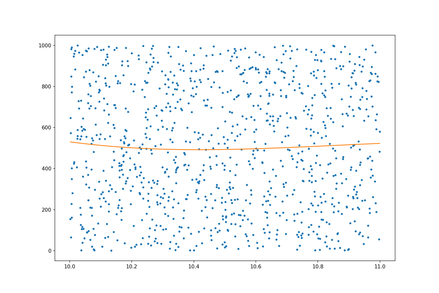
Fitting a single polynomial is fairly fast. In what follows, we test the runtime by fitting many polynomials:

>>> with Timer():
>>>     # Do the calculation for the 1000 groups of points.
>>>     polygroup = np.empty((1000, 3), dtype='float64')
>>>     for i in range(1000):
>>>         # Use numpy to build the point group.
>>>         slct = (xdata>=i)&(xdata<(i+1))
>>>         sub_x = xdata[slct]
>>>         sub_y = ydata[slct]
>>>         polygroup[i,:] = data_prep.fit_poly(sub_x, sub_y, 2)
Wall time: 1.49671 s

To analyze, we separate the house-keeping code outside the calculating helper:

>>> with Timer():
>>>     # Using numpy to build the point groups takes a lot of time.
>>>     data_groups = []
>>>     for i in range(1000):
>>>         slct = (xdata>=i)&(xdata<(i+1))
>>>         data_groups.append((xdata[slct], ydata[slct]))
Wall time: 1.24653 s

The real fitting code:

>>> with Timer():
>>>     # Fitting helper runtime is much less than building the point groups.
>>>     polygroup = np.empty((1000, 3), dtype='float64')
>>>     for it, (sub_x, sub_y) in enumerate(data_groups):
>>>         polygroup[it,:] = data_prep.fit_poly(sub_x, sub_y, 2)
Wall time: 0.215859 s

Although the house-keeping code is much easier to write in Python than in C++, it runs more than 5 times slower (the fitting code takes only 17% of the runtime of the house-keeping code).

Prepare Data in C++

Now run the C++ multi-polynomial helper. It detects the point group right before fitting:

>>> with Timer():
>>>     rbatch = data_prep.fit_polys(xdata, ydata, 2)
Wall time: 0.21058 s

The overhead of the Python house-keeping code is all gone.

SimpleArray

It has been shown that array is important for high-performance code. It is commonplace to develop a home-brewed array library for your system in C++, because it does not only provide general array operations, but also a place to house the ad hoc optimization that is crucial to performance.

In the above code we use a class template named SimpleArray. It is a header-only library that provides multi-dimensional accessors to a contiguous memory buffer. The primary use case is for fundamental numerical types. It has the following behaviors:

• Multi-dimensional access to regular memory buffers

• Simple memory allocation by using fixed size

• Separate buffer ownership and meta data

SimpleArray makes available the basic array meta data: shape, stride, and type. In addition to a spcific application, it also allows ghost (negative) index in the first dimension.

Note

A comparison between SimpleArray and the C++ std::vector is made below in the table Comparison between SimpleArray and C++ Vector.

Comparison between SimpleArray and C++ Vector

SimpleArray	std::vector
Fixed size (length): * Only allocate memory on construction	Variable size (length): * Buffer may be invalidated * Implicit memory allocation (reallocation)
Multi-dimensional access * Use operator()	One-dimensional access * Use operator[]

While the STL container std::vector is frequently used as a one-dimensional array of dynamic memory allocation, it does not have the exact capability and limitation that we want for high-performance code.

std::vector is definitely a powerful container. But its flexbility sometimes slows down the system or makes it harder to control. SimpleArray fills in the gap.

Buffer Ownership

SimpleArray uses a class ConcreteBuffer to manage the memory buffer, as shown below in the listing SimpleArray uses ConcreteBuffer to Manage Buffer:

SimpleArray uses ConcreteBuffer to Manage Buffer

template <typename T>
class SimpleArray
{
    using buffer_type = ConcreteBuffer;
    std::shared_ptr<buffer_type> m_buffer;
};

ConcreteBuffer itself is a class managed by std::shared_ptr:

class ConcreteBuffer
    : public std::enable_shared_from_this<ConcreteBuffer>
{
private:
    // Protect the constructors
    struct ctor_passkey {};

public:
    static std::shared_ptr<ConcreteBuffer> construct(size_t nbytes)
    {
        return std::make_shared<ConcreteBuffer>(nbytes, ctor_passkey());
    }

    ...
};

We would like to turn off the move semantics so that the memory controlled by ConcreteBuffer is not moved away unexpectedly:

// Turn off move
ConcreteBuffer(ConcreteBuffer &&) = delete;
ConcreteBuffer & operator=(ConcreteBuffer &&) = delete;

To make it possible to control when the memory controlled by ConcreteBuffer may be released, it internally is implemented by using std::unique_ptr and a custom deleter class:

// Use a deleter to customize memory management with unique_ptr
using data_deleter_type = detail::ConcreteBufferDataDeleter;
using unique_ptr_type = std::unique_ptr<int8_t, data_deleter_type>;

size_t m_nbytes;  // Remember the amount of bytes
unique_ptr_type m_data;  // Point to the allocated momery

Memory allocation is done in the constructor:

ConcreteBuffer(size_t nbytes, const ctor_passkey &)
    : m_nbytes(nbytes)
    , m_data(allocate(nbytes))
{}

// Allocate memory
static unique_ptr_type allocate(size_t nbytes)
{
    unique_ptr_type ret(nullptr, data_deleter_type());
    if (0 != nbytes)
    {
        ret = unique_ptr_type(new int8_t[nbytes], data_deleter_type());
    }
    return ret;
}

ConcreteBuffer Remover

The deleter ConcreteBufferDataDeleter is a proxy to a polymorphic remover functor type ConcreteBufferRemover:

struct ConcreteBufferDataDeleter
{
    using remover_type = ConcreteBufferRemover;
    explicit ConcreteBufferDataDeleter(std::unique_ptr<remover_type> && remover_in)
        : remover(std::move(remover_in))
    {}
    void operator()(int8_t * p) const
    {
        if (!remover)
        {
            delete[] p;  // Array deletion if no remover is available.
        }
        else
        {
            (*remover)(p);
        }
    }
    std::unique_ptr<remover_type> remover{nullptr};
};

The base class and the default implementation of ConcreteBufferRemover also uses the array deletion:

struct ConcreteBufferRemover
{
    virtual ~ConcreteBufferRemover() = default;
    virtual void operator()(int8_t * p) const
    {
        delete[] p;
    }
};

It may be customized to avoid releasing memory. When using ConcreteBuffer to hold pointer to a memory buffer managed by another sub-system, we may need to avoid releasing the memory when ConcreteBuffer destructs.

struct ConcreteBufferNoRemove : public ConcreteBufferRemover
{
    void operator()(int8_t *) const override {}
};

The full code is in ConcreteBuffer.hpp.

Multi-Dimensional Data Access

Three basic meta data are stored in SimpleArray to support multi-dimensional data access: shape, stride, and type. The type information is provided by the template argument. We do not need to pay a lot of attention to it.

template <typename T>
class SimpleArray
{
public:
    // Type information.
    using value_type = T;
    static constexpr size_t ITEMSIZE = sizeof(value_type);

    using buffer_type = ConcreteBuffer;
    /// Contiguous data buffer for the array.
    std::shared_ptr<buffer_type> m_buffer;

    using shape_type = small_vector<size_t>;
    /// Each element in this vector is the number of element in the
    /// corresponding dimension.
    shape_type m_shape;
    /// Each element in this vector is the number of elements (not number of
    /// bytes) to skip for advancing an index in the corresponding dimension.
    shape_type m_stride;
};

Shape describes the number of elements in each of the dimension of the array. In a one-dimensional array, the shape has only one element:

explicit SimpleArray(size_t length)
    : m_buffer(buffer_type::construct(length * ITEMSIZE))
    , m_shape{length}
    , m_stride{1}
    , m_body(m_buffer->data<T>())
{}

The size of the shape vector is the number of dimensionality:

explicit SimpleArray(shape_type const & shape)
    : m_shape(shape)
    , m_stride(calc_stride(m_shape))
{
    if (!m_shape.empty())
    {
        m_buffer = buffer_type::construct(m_shape[0] * m_stride[0] * ITEMSIZE);
        m_body = m_buffer->data<T>();
    }
}

Stride is the number of elements to be skipped when the index is changed by 1 in the corresponding dimension. The calculation is done by calc_stride().

static shape_type calc_stride(shape_type const & shape)
{
    shape_type stride(shape.size());
    if (!shape.empty())
    {
        stride[shape.size() - 1] = 1;
        for (size_t it = shape.size() - 1; it > 0; --it)
        {
            stride[it - 1] = stride[it] * shape[it];
        }
    }
    return stride;
}

Now the shape and stride are determined, and will be used in the multi-dimensional accessor. The accessor is broken into the element accessor in the form of operator()() and pointer accessor vptr(). When getting the address of an element, the pointer accessor is handy.

template <typename T>
class SimpleArray
{
    ...
    template <typename... Args>
    value_type const & operator()(Args... args) const
    { return *vptr(args...); }
    template <typename... Args>
    value_type & operator()(Args... args)
    { return *vptr(args...); }

    template <typename... Args>
    value_type const * vptr(Args... args) const
    { return m_body + buffer_offset(m_stride, args...); }
    template <typename... Args>
    value_type * vptr(Args... args)
    { return m_body + buffer_offset(m_stride, args...); }
    ...
};

SimpleArray uses the variadic template to get the indices in each of the dimensions and calculate the memory offset of the specified element. The helper template buffer_offset() is used to avoid conditioned branching in runtime.

namespace detail
{
// Use recursion in templates.
template <size_t D, typename S>
size_t buffer_offset_impl(S const &)
{
    return 0;
}
template <size_t D, typename S, typename Arg, typename... Args>
size_t buffer_offset_impl(S const & strides, Arg arg, Args... args)
{
    return arg * strides[D] +
           buffer_offset_impl<D + 1>(strides, args...);
}
} /* end namespace detail */

template <typename S, typename... Args>
size_t buffer_offset(S const & strides, Args... args)
{
    return detail::buffer_offset_impl<0>(strides, args...);
}

To this point, we will be able to access the elements using operator()():

SimpleArray<int> arr(small_vector<size_t>{3, 4});
arr_int(1, 2) = -8;

The full code is in SimpleArray.hpp.

Small Vector Optimization

For implmenting the shape and stride, SimpleArray employs the small vector optimization. When using arrays it is actually rare to use very high dimensions, e.g., 6. Instead, 1, 2, and 3 dimensions are the majority of the use cases. As we know dynamic allocation is expensive, it is good to spend a little bit of memory space to reduce the runtime overhead.

The optimization is to use a small block of memory in the class template (small_vector). Instead of using pointers for size and capacity, unsigned integers are used to keep track of the number of elements.

template <typename T, size_t N = 3>
class small_vector
{
public:
    T const * data() const { return m_head; }
    T * data() { return m_head; }
private:
    T * m_head = nullptr;
    unsigned int m_size = 0;
    unsigned int m_capacity = N;
    std::array<T, N> m_data;
};

Upon construction, if the requested size is smaller than N, no dynamic memory allocation is done:

explicit small_vector(size_t size)
    : m_size(static_cast<unsigned int>(size))
{
    if (m_size > N)
    {
        m_capacity = m_size;
        // Allocate only when the size is too large.
        m_head = new T[m_capacity];
    }
    else
    {
        m_capacity = N;
        m_head = m_data.data();
    }
}

small_vector() { m_head = m_data.data(); }

No deallocation is needed in the destructor if there was not dynamic memory used:

~small_vector()
{
    if (m_head != m_data.data() && m_head != nullptr)
    {
        delete[] m_head;
        m_head = nullptr;
    }
}

Copy constructor (as well as copy assignment operator, which is omitted here for clarity) may also allocate memory:

small_vector(small_vector const & other)
    : m_size(other.m_size)
{
    if (other.m_head == other.m_data.data())
    {
        m_capacity = N;
        m_head = m_data.data();
    }
    else
    {
        m_capacity = m_size;
        m_head = new T[m_capacity];
    }
    std::copy_n(other.m_head, m_size, m_head);
}

The move constructor (and move assignment operator, which is omitted here for clarity) should not allocate memory, but should take the

small_vector(small_vector && other) noexcept
    : m_size(other.m_size)
{
    if (other.m_head == other.m_data.data())
    {
        m_capacity = N;
        std::copy_n(other.m_data.begin(), m_size, m_data.begin());
        m_head = m_data.data();
    }
    else
    {
        m_capacity = m_size;
        m_head = other.m_head;
        other.m_size = 0;
        other.m_capacity = N;
        other.m_head = other.m_data.data();
    }
}

The full code is in small_vector.hpp.

Ghost (Negative) Index

Normally we access the element in an array using non-negative indices. But just like the C-style POD array, it is not wrong to allow negative indices as long as we do not access the memory out of the bound. It is a common trick played for implementing lookup tables.

To avoid incurring overhead for a normal array whose index starts with 0, SimpleArray implement the feature with only the leading dimension. What we need to do is to add the number of ghost elements (indexed using negative integer) and the starting address of the “non-ghost” body elements.

template <typename T>
class SimpleArray
{
private:
    // Number of ghost elements
    size_t m_nghost = 0;
    // Starting address of non-ghost
    value_type * m_body = nullptr;
};

The body address is calculated based on the data pointer, stride, and the ghost number:

static T * calc_body(T * data, shape_type const & stride, size_t nghost)
{
    if (nullptr == data || stride.empty() || 0 == nghost)
    {
        // Do nothing.
    }
    else
    {
        shape_type shape(stride.size(), 0);
        shape[0] = nghost;
        data += buffer_offset(stride, shape);
    }
    return data;
}

The ghost number and body address are calculated and assigned upon construction, e.g., in the copy and move constructors:

SimpleArray(SimpleArray const & other)
    : m_buffer(other.m_buffer->clone())
    , m_shape(other.m_shape)
    , m_stride(other.m_stride)
    , m_nghost(other.m_nghost)
    , m_body(calc_body(m_buffer->data<T>(), m_stride, other.m_nghost))
{}

SimpleArray(SimpleArray && other) noexcept
    : m_buffer(std::move(other.m_buffer))
    , m_shape(std::move(other.m_shape))
    , m_stride(std::move(other.m_stride))
    , m_nghost(other.m_nghost)
    , m_body(other.m_body)
{}

AOS and SOA

To write code for arrays, i.e., contiguous buffers of data, we go with either AOS (array of structures) or SOA (structure of arrays). As a rule of thumb, AOS is easier to code and SOA is more friendly to SIMD. However, it is not true that SOA is always faster than AOS [5] [6].

The demonstration of AOS and SOA here is elementary. Benchmarking the two different layouts is usually infeasible for a non-trivial system.

Array of Structures

AOS is commonplace in object-oriented programming that encourages encapsulating logic with data. Even though SOA is more friendly to memory access, the productivity of encapsulation makes it a better choice to start the system implementation.

Array of structures.

struct Point
{
    double x, y;
};

/**
 * Use a contiguous buffer to store the struct data element.
 */
using ArrayOfStruct = std::vector<Point>;

Structure of Arrays

In the following example code, each of the fields of a point is collected into the corresponding container in a structure StructOfArray.

It is not a good idea to expose the layout of the data, which is considered implementation detail. To implement the necessary encapsulation, we will need a handle or proxy class to access the point data.

Structure of arrays.

/**
 * In a real implementation, this data class needs encapsulation too.
 */
struct StructOfArray
{
    std::vector<double> x;
    std::vector<double> y;
};

/**
 * Because the data is "pool" in StructOfArray, it takes a handle or proxy
 * object to access the content point.
 */
struct PointHandle
{
    StructOfArray * soa;
    size_t idx;
    double   x() const { return soa.x[idx]; }
    double & x()       { return soa.x[idx]; }
    double   y() const { return soa.y[idx]; }
    double & y()       { return soa.y[idx]; }
};

Translation between Dynamic and Static

In C++ we can use template to do many things during compile time without needing to use a CPU instruction during runtime. For example, we may use CRTP (see Curiously Recursive Template Pattern (CRTP)) for the static polymorphism, instead of really checking for the type during runtime (dynamically).

But when we are trying to present the nicely optimized code to Python users, there is a problem: a dynamic language like Python does not know anything about a compile time entity like template. In Python, everything is dynamic (happens during runtime). We need to translate between the dynamic behaviors in Python and the static behaviors in C++.

This translation matters to our system design using arrays because the arrays carry type information that helps the C++ compiler generate efficient executables, and we do not want to lose the performance when doing the translation. Thus, it is not a bad idea to do it manually. Spelling out the static to dynamic conversion makes it clear what do we want to do. When we work in the inner-most loop, no PyObject or virtual function table should be there. The explicitness will help us add ad hoc optimization or debug for difficult performance issues.

We will use an example to show one way to explicitly separate the static and dynamic behaviors. The model problem is to define the operations of the spatially discretized grid and the elements.

Class Templates for General Behaviors

There should be general code and information for all of the grids, and they are kept in some class templates. The C++ compiler knows when to put the code and information in proper places.

The (static) class template for grids.

/**
 * Spatial table basic information.  Any table-based data store for spatial
 * data should inherit this class template.
 */
template <size_t ND>
class SpaceBase
{
public:
    static constexpr const size_t NDIM = ND;
    using serial_type = uint32_t;
    using real_type = double;
};

/**
 * Base class template for structured grid.
 */
template <dim_t ND>
class StaticGridBase
  : public SpaceBase<ND>
{
    // Code that is general to the grid of any dimension.
};

Classes for Specific Behaviors

There may be different behaviors for each of the dimension, and we may use a class to house the code and data.

The classes instantiating the grid class templates.

class StaticGrid1d
  : public StaticGridBase<1>
{
};

class StaticGrid2d
  : public StaticGridBase<2>
{
};

class StaticGrid3d
  : public StaticGridBase<3>
{
};

Dynamic Behaviors in Interpreter

Everything in Python needs to be dynamic, and we can absorb it in the wrapping layer.

The ad hoc wrappers for each of the grid classes.

/*
 * WrapStaticGridBase has the pybind11 wrapping code.
 */

class WrapStaticGrid1d
  : public WrapStaticGridBase< WrapStaticGrid1d, StaticGrid1d >
{
};

class WrapStaticGrid2d
  : public WrapStaticGridBase< WrapStaticGrid2d, StaticGrid2d >
{
};

class WrapStaticGrid3d
  : public WrapStaticGridBase< WrapStaticGrid3d, StaticGrid3d >
{
};

PYBIND11_MODULE(_modmesh, mod)
{
    WrapStaticGrid1d::commit(mod);
    WrapStaticGrid2d::commit(mod);
    WrapStaticGrid3d::commit(mod);
}

How pybind11 Translates

We rely on pybind11 for doing the translate behind the wrappers.

Here we take a look at the code of a older version 2.4.3 to understand what is happening behind the scenes. pybind11 uses the class pybind11::cppfunction to wrap everything that is callable in C++ to be a callable in Python (see line 56 in pybind11.h):

/// Wraps an arbitrary C++ function/method/lambda function/.. into a callable Python object
class cpp_function : public function {
public:
    cpp_function() { }
    cpp_function(std::nullptr_t) { }

    /// Construct a cpp_function from a vanilla function pointer
    template <typename Return, typename... Args, typename... Extra>
    cpp_function(Return (*f)(Args...), const Extra&... extra) {
        initialize(f, f, extra...);
    }

    /// Construct a cpp_function from a lambda function (possibly with internal state)
    template <typename Func, typename... Extra,
              typename = detail::enable_if_t<detail::is_lambda<Func>::value>>
    cpp_function(Func &&f, const Extra&... extra) {
        initialize(std::forward<Func>(f),
                   (detail::function_signature_t<Func> *) nullptr, extra...);
    }

    /// Construct a cpp_function from a class method (non-const)
    template <typename Return, typename Class, typename... Arg, typename... Extra>
    cpp_function(Return (Class::*f)(Arg...), const Extra&... extra) {
        initialize([f](Class *c, Arg... args) -> Return { return (c->*f)(args...); },
                   (Return (*) (Class *, Arg...)) nullptr, extra...);
    }

    /// Construct a cpp_function from a class method (const)
    template <typename Return, typename Class, typename... Arg, typename... Extra>
    cpp_function(Return (Class::*f)(Arg...) const, const Extra&... extra) {
        initialize([f](const Class *c, Arg... args) -> Return { return (c->*f)(args...); },
                   (Return (*)(const Class *, Arg ...)) nullptr, extra...);
    }

// ...
}

The constructors call pybind11::cppfunction::initialize() to populate necessary information for the callables: to be a callable in Python (see line 98 in pybind11.h):

/// Special internal constructor for functors, lambda functions, etc.
template <typename Func, typename Return, typename... Args, typename... Extra>
void initialize(Func &&f, Return (*)(Args...), const Extra&... extra) {
  // Code populating necessary information for calling the callables.
}

When Python wants to call a callable controlled by pybind11::cppfunction, pybind11 uses pybind11::cppfunction::dispatch() to find the corresponding object (see line 423 in pybind11.h):

static PyObject *dispatcher(PyObject *self, PyObject *args_in, PyObject *kwargs_in) {
  // Read the Python information and find the right cppfunction for execution.
}

Scoped-Based Timer

Profiling is the first thing to do when we need to optimize the code we write. While profiling itself has nothing specific to array code, it is common for us to consider profiling along with writing the high-performance array-style code, because both are meant for improving the system performance.

In addition to using OS-provided profiling tools, e.g., Linux’s perf and Macos’s Instruments, we should also add a custom profiling layer in the code. We usually use a simple scope-based profiler for ease of implementation, but sample-based works as well.

The custom profiler is especially useful in two scenarios:

1. The destination platform does not have a very good profiler.

2. We may not access to a system profiler for some reasons (permission, accessibility, etc.)

Even though a custom profiler may not use the most delicate implementation, it is the last thing you may rely on. Another benefit of using a custom profiler is that you may add code specific to your applications, which is usually infeasible for a general profiler.

The following example implements a simple scoped-based timer that is controlled by a pre-processor macro:

A simple scoped-based timer in C++.

/*
 * MODMESH_PROFILE defined: Enable profiling API.
 */
#ifdef MODMESH_PROFILE

#define MODMESH_TIME(NAME) \
    ScopedTimer local_scoped_timer_ ## __LINE__(NAME);

/*
 * No MODMESH_PROFILE defined: Disable profiling API.
 */
#else // MODMESH_PROFILE

#define MODMESH_TIME(NAME)

#endif // MODMESH_PROFILE
/*
 * End MODMESH_PROFILE.
 */

struct ScopedTimer
{

    ScopedTimer() = delete;

    ScopedTimer(const char * name) : m_name(name) {}

    ~ScopedTimer()
    {
        TimeRegistry::me().add(m_name, m_sw.lap());
    }

    StopWatch m_sw;
    char const * m_name;

}; /* end struct ScopedTimer */

This is the usage example:

Use the simple timer.

// Manually
void StaticGrid1d::fill(StaticGrid1d::real_type val)
{
    MODMESH_TIME("StaticGrid1d::fill");
    std::fill(m_coord.get(), m_coord.get()+m_nx, val);
}

The system provides a way to keep and print the timing data (see the code elsewhere):

>>> import modmesh as mm
>>>
>>> gd = mm.StaticGrid1d(1000000)
>>> for it in range(100):
>>>     gd.fill(0)
>>> print(mm.time_registry.report())
StaticGrid1d.__init__ : count = 1 , time = 6.36e-06 (second)
StaticGrid1d.fill : count = 100 , time = 0.0346712 (second)
StaticGrid1d::fill : count = 100 , time = 0.0344818 (second)

Note

There are many ways to do a custom profiler. Another good way to do it is to add one at the pybind11 wrapping layer. Python function calls are much more expensive than C++ ones. Adding timers when calling from Python to C++ never makes a dent to the overall runtime.

Exercises

1. By allowing changing the signature of the function fit_poly(), how can we ensure the shapes of xarr and yarr to be the same, without the explicit check with "xarr and yarr size mismatch"? Write code to show.

References

[1]

Example Code: C++ and C for Python

[2]

modmesh: https://github.com/solvcon/modmesh

[3]

pybind11 Seamless operability between C++11 and Python: https://pybind11.readthedocs.io/en/stable/

[4]

IPython / Jupyter integration for pybind11: https://github.com/aldanor/ipybind

[5]

Memory Layout Transformations: https://software.intel.com/content/www/us/en/develop/articles/memory-layout-transformations.html

[6]

Chapter 31 - Abstraction for AoS and SoA Layout in C++, GPU Computing Gems Jade Edition, pp. 429-441, Robert Strzodka, January 1, 2012. http://www.sciencedirect.com/science/article/pii/B9780123859631000319