Matrix Operations

System should be designed as simple as possible. Any excessive complexity slows it down. This is why we use arrays so frequently when it comes to designing a high-performance system. Array is the data structure closest to the fundamental types, and the hardware knows how to process the data quickly in batch. By making the data complex, we will force the computers to take more time to mitigate our laziness.

In numerical analysis, the counterpart of array is matrix. It is coincident that matrices are so useful to a wide range of real-world problems, but it is undeniable that computers extend the application to an unbelievable scale. It probably has something to do with the linearity of human minds, but don’t quote me on the anecdotal statement.

Linear Algebra

One of the most frequent use of matrices is linear algebra. BLAS [2] and LAPACK [3] are the two most important libraries for numerical calculations for linear algebra. BLAS stands for Basic Linear Algebra Subprograms, and LAPACK is Linear Algebra PACKage. They were originally developed in Fortran. The Fortran code is still being maintained today, and serves as a reference implementation. Production code is encouraged to use the vendor-optimized implementation, e.g., Intel’s Math Kernel Library (MKL) [4], Apple’s Accelerate/vecLib [5], etc.

BLAS is organized at 3 levels:

• Level 1 is vector operations, e.g.,

  • SAXPY(): \(\mathbf{y} = a\mathbf{x} + \mathbf{y}\), constant times a vector plus a vector.

  • SDOT(): \(\mathbf{x}\cdot\mathbf{y}\), dot product of two vectors.

  • SNRM2(): \(\sqrt{\mathbf{y}\cdot\mathbf{y}}\), Euclidean norm.

• Level 2 is matrix-vector operations, e.g.,

  • SGEMV(): \(\mathbf{y} = \alpha\mathrm{A}\mathbf{x} + \beta\mathbf{y}\), performs the general matrix-vector multiplication.

• Level 3 is matrix-matrix operations, e.g.,

  • SGEMM(): \(\mathrm{C} = \alpha\mathrm{A}\mathrm{B} + \beta\mathrm{C}\), performs the general matrix-matrix multiplication.

Note

In the naming convention of BLAS, the leading character denotes the precision of the data that is to be processed. It may be one of S, D, C, and Z, for single-precision real, double-precision real, single-precision complex, and double-precision complex, respectively.

LAPACK is designed to rely on the underneath BLAS, so the two libraries are usually used together. While BLAS offers basic operations like matrix multiplication, LAPACK provides more versatile computation helpers or solvers, e.g., a system of linear equations, least square, and eigen problems.

Both BLAS and LAPACK provide C API (no native C++ interface). CBLAS is the C API for BLAS and CLAPACK and LAPACKE are that for LAPACK.

POD Arrays

The plain-old-data (POD) arrays are also called C-style arrays. They are given the names because they are nothing more than just plain buffers in memory and support no mechanism fancier than that. We do, oftentimes, wrap POD with fancy C++ constructs, but the underneath heavy-lifting calculations still deal with POD directly. (It clearly reveals itself in the machine code.)

Vector: 1D Array

We may use a 1D array (a contiguous memory buffer of sequentially ordered elements) to store a vector. Small vectors may be created on the stack:

constexpr size_t width = 5;
double vector[width];

It can be indexed and populated using the index:

// Populate a vector.
for (size_t i=0; i<width; ++i)
{
    vector[i] = i;
}

It is common to use the index to manipulate the 1-D array. The memory layout is:

The following code prints the contents:

std::cout << "vector elements in memory:" << std::endl << " ";
for (size_t i=0; i<width; ++i)
{
    std::cout << " " << vector[i];
}
std::cout << std::endl;

The execution results verify that the contents are following the depicted memory layout:

vector elements in memory:
  0 1 2 3 4

The full example code can be found in pod01_vector.cpp.

Matrix: 2D Array

In mathematics, we usually write a matrix like:

\[\begin{split}\mathrm{A} = \left[ a_{ij} \right] = \left(\begin{array}{ccccc} a_{11} & a_{12} & a_{13} & a_{14} & a_{15} \\ a_{21} & a_{22} & a_{23} & a_{24} & a_{25} \\ a_{31} & a_{32} & a_{33} & a_{34} & a_{35} \\ a_{41} & a_{42} & a_{43} & a_{44} & a_{45} \\ a_{51} & a_{52} & a_{53} & a_{54} & a_{55} \end{array}\right)\end{split}\]

It is a \(5\times5\) square matrix. \(i\) is the row index (in the horizontal direction). \(j\) is the column index (in the vertical direction).

However, computer code usually uses 0-based index, so the first index starts with 0, not 1. It would make coding easier to rewrite the matrix using the 0-based index:

\[\begin{split}\mathrm{A} = \left[ a_{ij} \right] = \left(\begin{array}{ccccc} a_{00} & a_{01} & a_{02} & a_{03} & a_{04} \\ a_{10} & a_{11} & a_{12} & a_{13} & a_{14} \\ a_{20} & a_{21} & a_{22} & a_{23} & a_{24} \\ a_{30} & a_{31} & a_{32} & a_{33} & a_{34} \\ a_{40} & a_{41} & a_{42} & a_{43} & a_{44} \end{array}\right)\end{split}\]

There is a simple and convenient way in C++ to handle the matrices and it is to use to following syntax:

constexpr size_t width = 5;

double amatrix[width][width];

The elements are accessed through two consecutive operators [][]:

// Populate the matrix on stack (row-major 2D array).
for (size_t i=0; i<width; ++i) // the i-th row
{
    for (size_t j=0; j<width; ++j) // the j-th column
    {
        amatrix[i][j] = i*10 + j;
    }
}

std::cout << "2D array elements:";
for (size_t i=0; i<width; ++i) // the i-th row
{
    std::cout << std::endl << " ";
    for (size_t j=0; j<width; ++j) // the j-th column
    {
        std::cout << " " << std::setfill('0') << std::setw(2)
                  << amatrix[i][j];
    }
}
std::cout << std::endl;

The execution results are:

2D array elements:
  00 01 02 03 04
  10 11 12 13 14
  20 21 22 23 24
  30 31 32 33 34
  40 41 42 43 44

The full example code can be found in pod02_matrix_auto.cpp.

But there is a caveat. The multi-dimensional array syntax only works with auto variable. That is what will be discussed next.

Variable-Length Array

The C++ multi-dimensional array index is convenient, but it doesn’t always work when the array size is unknown in the compile time, which is also known as variable-length arrays (VLA). VLA is included in the C standard [7], but not in the C++ standard.

g++ accepts the following code for GCC provides the VLA extension in C++:

void work(double * buffer, size_t width)
{
    // This should not work since width is unknown in compile time.
    double (*matrix)[width] = reinterpret_cast<double (*)[width]>(buffer);
    //...
}

clang++ doesn’t:

$ clang++ pod_bad_matrix.cpp -o pod_bad_matrix -std=c++17 -O3 -g -m64
pod_bad_matrix.cpp:7:14: error: cannot initialize a variable of type 'double (*)[width]' with an rvalue of type 'double (*)[width]'
    double (*matrix)[width] = reinterpret_cast<double (*)[width]>(buffer);
             ^                ~~~~~~~~~~~~~~~~~~~~~~~~~~~~~~~~~~~~~~~~~~~
1 error generated.
make: *** [pod_bad_matrix] Error 1

The full example code can be found in pod_bad_matrix.cpp.

In general, we should not use the simple multi-dimensional syntax when the size of the array is not known during compile time. If the memory offset needs to be determined during runtime, use syntax for obviously runtime behavior.

Row-Major 2D Array

A row-major 2D array makes the access of data in a matrix row to be contiguous:

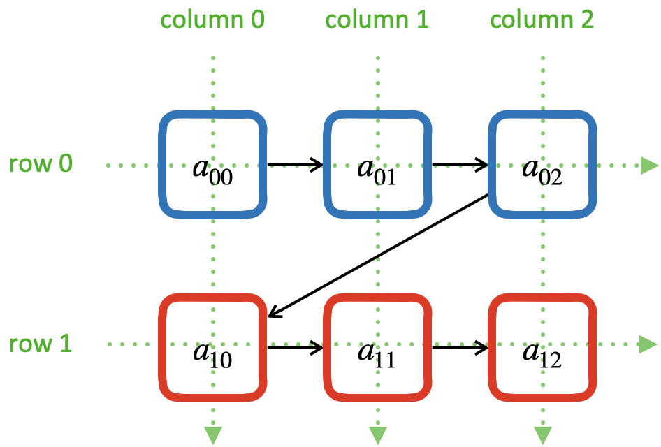
The elements of a row-major 2D array are stored so that the fastest changing index is the trailing index of the 2D array:

constexpr size_t width = 5;
double * buffer = new double[width*width];

\[\mathrm{buffer} = [a_{00}, a_{01}, a_{02}, a_{03}, a_{04}, a_{10}, a_{11}, a_{12}, \ldots, a_{43}, a_{44}]\]

When accessing the elements, what we need to do is to remember how long we need to stride per row (leading) index. In the above case, it is i*width. Then we can use the stride to calculate the correct index in the buffer (the following code populates the buffer):

// Populate a buffer (row-major 2D array).
for (size_t i=0; i<width; ++i) // the i-th row
{
    for (size_t j=0; j<width; ++j) // the j-th column
    {
        buffer[i*width + j] = i*10 + j;
    }
}

We may play the pointer trick (which didn’t work for VLA) to use two consecutive operators [][] for accessing the element:

// Make a pointer to double[width].  Note width is a constexpr.
double (*matrix)[width] = reinterpret_cast<double (*)[width]>(buffer);
std::cout << "matrix address: " << matrix << std::endl;

std::cout << "matrix (row-major) elements as 2D array:";
for (size_t i=0; i<width; ++i) // the i-th row
{
    std::cout << std::endl << " ";
    for (size_t j=0; j<width; ++j) // the j-th column
    {
        std::cout << " " << std::setfill('0') << std::setw(2)
                  << matrix[i][j];
    }
}
std::cout << std::endl;

The execution results are:

buffer address: 0x7f88e9405ab0
matrix address: 0x7f88e9405ab0
matrix (row-major) elements as 2D array:
  00 01 02 03 04
  10 11 12 13 14
  20 21 22 23 24
  30 31 32 33 34
  40 41 42 43 44
matrix (row-major) elements in memory:
  00 01 02 03 04 10 11 12 13 14 20 21 22 23 24 30 31 32 33 34 40 41 42 43 44
row majoring: the fastest moving index is the trailing index

The full example code can be found in pod03_matrix_rowmajor.cpp.

Column-Major 2D Array

A column-major 2D array makes the access of data in a matrix column to be contiguous:

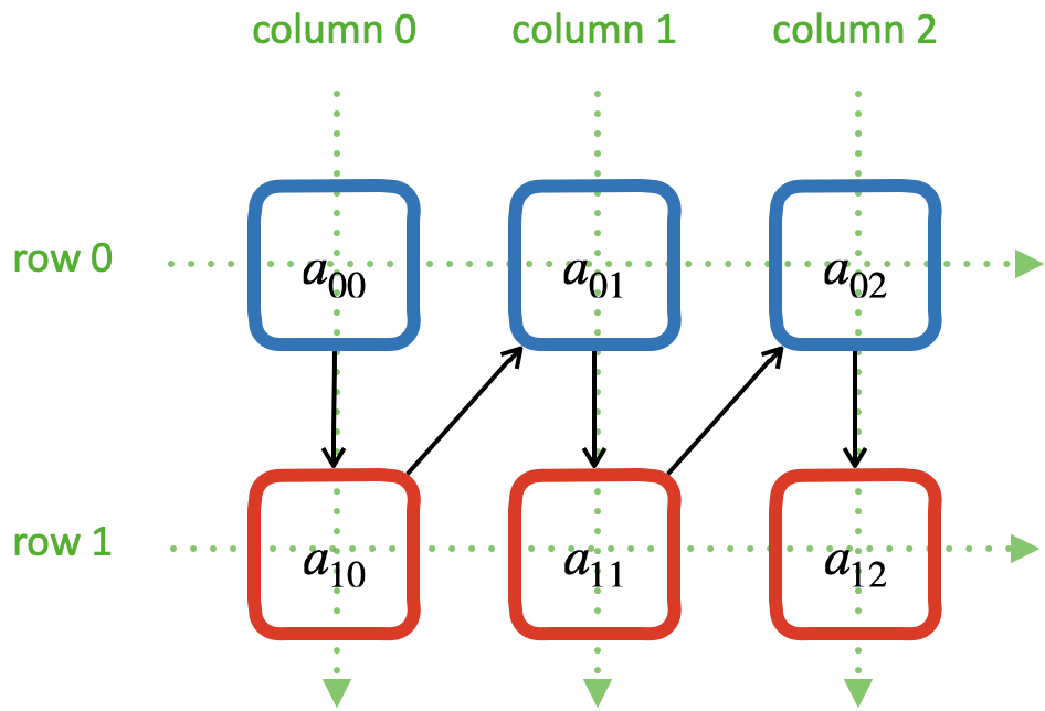
The elements of a column-major 2D array are stored so that the fastest changing index is the leading index of the 2D array:

constexpr size_t width = 5;
double * buffer = new double[width*width];

The above code is the same as that of the row-majoring since the number of column and row is the same. But for column-majoring arrays, the elements order differently:

\[\mathrm{buffer} = [a_{00}, a_{10}, a_{20}, a_{30}, a_{40}, a_{01}, a_{11}, a_{21}, \ldots, a_{34}, a_{44}]\]

Similar to a row-major array, we need to know the stride. But this time it’s for the column (trailing) index:

// Populate a buffer (column-major 2D array).
for (size_t i=0; i<width; ++i) // the i-th row
{
    for (size_t j=0; j<width; ++j) // the j-th column
    {
        buffer[j*width + i] = i*10 + j;
    }
}

The same pointer trick allows to use two consecutive operators [][], but it does not know the different stride needed by column-majoring, and does not work well. We need to flip i and j to hack out the column-major stride:

// Make a pointer to double[width].  Note width is a constexpr.
double (*matrix)[width] = reinterpret_cast<double (*)[width]>(buffer);
std::cout << "matrix address: " << matrix << std::endl;

std::cout << "matrix (column-major) elements as 2D array:";
for (size_t i=0; i<width; ++i) // the i-th row
{
    std::cout << std::endl << " ";
    for (size_t j=0; j<width; ++j) // the j-th column
    {
        std::cout << " " << std::setfill('0') << std::setw(2)
                  << matrix[j][i];
    }
}
std::cout << std::endl;

In the above code, to access the element \(a_{ij}\) (at i-th row and j-th column), the code needs to be written as matrix[j][i]. This does not look as straight-forward as that of the row-major array, which was matrix[i][j].

The execution results are:

buffer address: 0x7f926bc05ab0
matrix address: 0x7f926bc05ab0
matrix (column-major) elements as 2D array:
  00 01 02 03 04
  10 11 12 13 14
  20 21 22 23 24
  30 31 32 33 34
  40 41 42 43 44
matrix (column-major) elements in memory:
  00 10 20 30 40 01 11 21 31 41 02 12 22 32 42 03 13 23 33 43 04 14 24 34 44
column majoring: the fastest moving index is the leading index

The full example code can be found in pod04_matrix_colmajor.cpp.

C++ Class for Matrix

Keeping track of the stride can be error-prone. Even if we stick to one majoring order (usually it’s row-majoring), it’s easy to lose track of it when the number of row and column is different, or it’s higher-dimensional.

A common practice in C++ is to use a class to keep track of the stride and simply access:

class Matrix {

public:

    Matrix(size_t nrow, size_t ncol)
      : m_nrow(nrow), m_ncol(ncol)
    {
        size_t nelement = nrow * ncol;
        m_buffer = new double[nelement];
    }

    ~Matrix()
    {
        delete[] m_buffer;
    }

    // No bound check.
    double   operator() (size_t row, size_t col) const
    {
        return m_buffer[row*m_ncol + col];
    }
    double & operator() (size_t row, size_t col)
    {
        return m_buffer[row*m_ncol + col];
    }

    size_t nrow() const { return m_nrow; }
    size_t ncol() const { return m_ncol; }

private:

    size_t m_nrow;
    size_t m_ncol;
    double * m_buffer;

};

The key is the custom operator() added in lines 17–25. It uses the stride information stored in the object to index the correct element. The populating code is simplified by using the new accessor:

/**
 * Populate the matrix object.
 */
void populate(Matrix & matrix)
{
    for (size_t i=0; i<matrix.nrow(); ++i) // the i-th row
    {
        for (size_t j=0; j<matrix.ncol(); ++j) // the j-th column
        {
            matrix(i, j) = i*10 + j;
        }
    }
}

The execution results are:

matrix:
  00 01 02 03 04
  10 11 12 13 14
  20 21 22 23 24
  30 31 32 33 34
  40 41 42 43 44

The full example code can be found in ma01_matrix_class.cpp.

Matrix Transpose

Before other operations related to a 2D array, we should first discuss matrix transpose. Write a \(m\times n\) (\(m\) rows and \(n\) columns) matrix \(\mathrm{A}\)

\[\begin{split}\mathrm{A} = [a_{ij}] = \left(\begin{array}{cccc} a_{11} & a_{12} & \cdots & a_{1n} \\ a_{21} & a_{22} & \cdots & a_{2n} \\ a_{31} & a_{32} & \cdots & a_{3n} \\ \vdots & & \ddots & \vdots \\ a_{m1} & a_{m2} & \cdots & a_{mn} \end{array}\right)_{m\times n}\end{split}\]

its transpose \(\mathrm{A}^t\) becomes a \(n\times m\) (\(n\) rows and \(m\) columns) matrix

\[\begin{split}\mathrm{A}^t = [a_{ji}] = \left(\begin{array}{ccccc} a_{11} & a_{21} & a_{31} & \cdots & a_{m1} \\ a_{12} & a_{22} & a_{32} & \cdots & a_{m2} \\ \vdots & & & \ddots & \vdots \\ a_{1n} & a_{2n} & a_{3n} & \cdots & a_{mn} \end{array}\right)_{n\times m}\end{split}\]

In computer code, transposing may be implementing by creating two memory buffers and copy from the source to the destination. An alternate and faster approach is to take advantage of majoring.

The fast transpose uses the formula \(\mathrm{A}^t = [a_{ji}]\) for \(\mathrm{A} = [a_{ij}]\). The code is like:

double   operator() (size_t row, size_t col) const
{
    return m_buffer[index(row, col)];
}
double & operator() (size_t row, size_t col)
{
    return m_buffer[index(row, col)];
}

bool is_transposed() const { return m_transpose; }

Matrix & transpose()
{
    m_transpose = !m_transpose;
    std::swap(m_nrow, m_ncol);
    return *this;
}

There is no data copied for transpose. The price to pay is the if statement in the indexing helper.

size_t index(size_t row, size_t col) const
{
    if (m_transpose) { return row          + col * m_nrow; }
    else             { return row * m_ncol + col         ; }
}

Matrix-Vector Multiplication

Operations of a matrix and a vector make coding for matrices more interesting. To show how it works, let us use a concrete operation of matrix-vector multiplication

\[\mathbf{y} = \mathrm{A}\mathbf{x}\]

Come back to the matrix-vector multiplication, \(\mathbf{y} = \mathrm{A}\mathbf{x}\). The calculation is easy by using the index form of the matrix and vector.

\[y_i = \sum_{j=1}^n A_{ij} x_j, \quad i = 1, \ldots, m\]

By applying Einstein’s summation convention [8], the summation sign may be suppressed to use the repeated indices for summation

\[y_i = A_{ij} x_j, \quad i = 1, \ldots, m, \; j = 1, \ldots, n\]

It can be shown that the index form of \(\mathbf{y}' = \mathrm{A}^t\mathbf{x}'\) is

\[y'_j = A_{ji} x'_i, \quad i = 1, \ldots, m, \; j = 1, \ldots, n\]

Aided by the above equations, we may implement a naive matrix-vector multiplication:

std::vector<double> operator*(Matrix const & mat, std::vector<double> const & vec)
{
    if (mat.ncol() != vec.size())
    {
        throw std::out_of_range("matrix column differs from vector size");
    }

    std::vector<double> ret(mat.nrow());

    for (size_t i=0; i<mat.nrow(); ++i)
    {
        double v = 0;
        for (size_t j=0; j<mat.ncol(); ++j)
        {
            v += mat(i,j) * vec[j];
        }
        ret[i] = v;
    }

    return ret;
}

Full example code can be found in ma02_matrix_vector.cpp. In the rest of the section, we will analyze the multiplication code with several different configurations.

Square Matrix

First we test the simple case. Multiplying a \(5\times5\) square matrix by a \(5\times1\) vector:

size_t width = 5;

std::cout << ">>> square matrix-vector multiplication:" << std::endl;
Matrix mat(width, width);

for (size_t i=0; i<mat.nrow(); ++i) // the i-th row
{
    for (size_t j=0; j<mat.ncol(); ++j) // the j-th column
    {
        mat(i, j) = i == j ? 1 : 0;
    }
}

std::vector<double> vec{1, 0, 0, 0, 0};
std::vector<double> res = mat * vec;

std::cout << "matrix A:" << mat << std::endl;
std::cout << "vector b:" << vec << std::endl;
std::cout << "A*b =" << res << std::endl;

The result is a \(5\times1\) vector:

>>> square matrix-vector multiplication:
matrix A:
   1  0  0  0  0
   0  1  0  0  0
   0  0  1  0  0
   0  0  0  1  0
   0  0  0  0  1
vector b: 1 0 0 0 0
A*b = 1 0 0 0 0

Rectangular Matrix

Multiplying a \(2\times3\) square matrix by a \(3\times1\) vector:

std::cout << ">>> m*n matrix-vector multiplication:" << std::endl;
Matrix mat2(2, 3);

double v = 1;
for (size_t i=0; i<mat2.nrow(); ++i) // the i-th row
{
    for (size_t j=0; j<mat2.ncol(); ++j) // the j-th column
    {
        mat2(i, j) = v;
        v += 1;
    }
}

std::vector<double> vec2{1, 2, 3};
std::vector<double> res2 = mat2 * vec2;

std::cout << "matrix A:" << mat2 << std::endl;
std::cout << "vector b:" << vec2 << std::endl;
std::cout << "A*b =" << res2 << std::endl;

The result is a \(2\times1\) vector:

>>> m*n matrix-vector multiplication:
matrix A:
   1  2  3
   4  5  6
vector b: 1 2 3
A*b = 14 32

Transposed Matrix

Apply the fast transpose to the \(2\times3\) square matrix mat2 to make it a \(3\times2\) matrix, and multiply by a \(2\times1\) vector:

std::cout << ">>> transposed matrix-vector multiplication:" << std::endl;
mat2.transpose();
std::vector<double> vec3{1, 2};
std::vector<double> res3 = mat2 * vec3;

std::cout << "matrix A:" << mat2 << std::endl;
std::cout << "matrix A buffer:" << mat2.buffer_vector() << std::endl;
std::cout << "vector b:" << vec3 << std::endl;
std::cout << "A*b =" << res3 << std::endl;

The result is a \(3\times1\) vector:

>>> transposed matrix-vector multiplication:
matrix A:
   1  4
   2  5
   3  6
matrix A buffer: 1 2 3 4 5 6
vector b: 1 2
A*b = 9 12 15

Because of the transpose, the matrix now uses column-majoring, as shown in the sixth line in the result above.

New Buffer from Transpose

Also try to copy the transposed matrix to a new matrix object which uses a new buffer. Multiply the new matrix with the same vector:

std::cout << ">>> copied transposed matrix-vector multiplication:" << std::endl;
Matrix mat3 = mat2;
res3 = mat3 * vec3;

std::cout << "matrix A:" << mat3 << std::endl;
std::cout << "matrix A buffer:" << mat3.buffer_vector() << std::endl;
std::cout << "vector b:" << vec3 << std::endl;
std::cout << "A*b =" << res3 << std::endl;

The copy assignment operator is implemented as:

Matrix & operator=(Matrix const & other)
{
    if (this == &other) { return *this; }
    if (m_nrow != other.m_nrow || m_ncol != other.m_ncol)
    {
        reset_buffer(other.m_nrow, other.m_ncol);
    }
    for (size_t i=0; i<m_nrow; ++i)
    {
        for (size_t j=0; j<m_ncol; ++j)
        {
            (*this)(i,j) = other(i,j);
        }
    }
    return *this;
}

The result is the same \(3\times1\) vector:

>>> copied transposed matrix-vector multiplication:
matrix A:
   1  4
   2  5
   3  6
matrix A buffer: 1 4 2 5 3 6
vector b: 1 2
A*b = 9 12 15

The copied matrix uses row-majoring, as shown in the sixth line in the result above.

Note

Although we do not analyze the runtime performance at this moment, the majoring may significantly affects the speed of the multiplication for large matrices.

Matrix-Matrix Multiplication

Matrix-matrix multiplication, \(\mathrm{C} = \mathrm{A}\mathrm{B}\), has more complexity in both time and space. It generally uses a \(O(n^3)\) algorithm for multiple copies of \(O(n^2)\) data. The formula is

\[C_{ik} = \sum_{j=1}^n A_{ij}B_{jk}, \quad i = 1, \ldots, m, \; k = 1, \ldots, l\]

or, by using Einstein’s summation convention,

\[C_{ik} = A_{ij}B_{jk}, \quad i = 1, \ldots, m, \; j = 1, \ldots, n, \; k = 1, \ldots, l\]

Aided by the formula, we can write down the C++ code for the naive algorithm:

Matrix operator*(Matrix const & mat1, Matrix const & mat2)
{
    if (mat1.ncol() != mat2.nrow())
    {
        throw std::out_of_range(
            "the number of first matrix column "
            "differs from that of second matrix row");
    }

    Matrix ret(mat1.nrow(), mat2.ncol());

    for (size_t i=0; i<ret.nrow(); ++i)
    {
        for (size_t k=0; k<ret.ncol(); ++k)
        {
            double v = 0;
            for (size_t j=0; j<mat1.ncol(); ++j)
            {
                v += mat1(i,j) * mat2(j,k);
            }
            ret(i,k) = v;
        }
    }

    return ret;
}

The 3-level nested loops in lines 12–23 are the runtime hotspot. The full example code can be found in ma03_matrix_matrix.cpp. We will examine two cases. The first is to multiply a \(2\times3\) matrix \(\mathrm{A}\) by a \(3\times2\) matrix \(\mathrm{B}\):

std::cout << ">>> A(2x3) times B(3x2):" << std::endl;
Matrix mat1(2, 3, std::vector<double>{1, 2, 3, 4, 5, 6});
Matrix mat2(3, 2, std::vector<double>{1, 2, 3, 4, 5, 6});

Matrix mat3 = mat1 * mat2;

std::cout << "matrix A (2x3):" << mat1 << std::endl;
std::cout << "matrix B (3x2):" << mat2 << std::endl;
std::cout << "result matrix C (2x2) = AB:" << mat3 << std::endl;

The result is a \(2\times2\) matrix \(\mathrm{C}\):

>>> A(2x3) times B(3x2):
matrix A (2x3):
   1  2  3
   4  5  6
matrix B (3x2):
   1  2
   3  4
   5  6
result matrix C (2x2) = AB:
  22 28
  49 64

Then multiply \(\mathrm{B}\) (\({3\times2}\)) by \(\mathrm{A}\) (\({2\times3}\)):

std::cout << ">>> B(3x2) times A(2x3):" << std::endl;
Matrix mat4 = mat2 * mat1;
std::cout << "matrix B (3x2):" << mat2 << std::endl;
std::cout << "matrix A (2x3):" << mat1 << std::endl;
std::cout << "result matrix D (3x3) = BA:" << mat4 << std::endl;

The result is a \(3\times3\) matrix \(\mathrm{D}\):

>>> B(3x2) times A(2x3):
matrix B (3x2):
   1  2
   3  4
   5  6
matrix A (2x3):
   1  2  3
   4  5  6
result matrix D (3x3) = BA:
   9 12 15
  19 26 33
  29 40 51

Matrix-matrix multiplication is intensive number-crunching. We do not have a good way to work around the brute-force, N-cube algorithm.

Note

An algorithm of slightly lower complexity in time is available [9], but not discussed here. We use the naive algorithm to focus the discussions on the code development.

It also demands memory. A matrix of \(100,000\times100,000\) takes 10,000,000,000 (i.e., \(10^{10}\)) elements, and with double-precision floating points, it takes 80 GB. To perform multiplication, you need the memory for 3 of the matrices, and that’s 240 GB. The dense matrix multiplication does not scale well with distributed-memory parallelism. The reasonable size of dense matrices for a workstation is around \(10,000\times10,000\), i.e., 800 MB per matrix. It’s very limiting, but already facilitates a good number of applications.

Linear System

LAPACK provides ?GESV() functions to solve a linear system using a general (dense) matrix: \(\mathrm{A}\mathbf{x} = \mathbf{b}\). Say we have a system of linear equations:

\[\begin{split}3 x_1 + 5 x_2 + 2 x_3 &= 57 \\ 2 x_1 + x_2 + 3 x_3 &= 22 \\ 4 x_1 + 3 x_2 + 2 x_3 &= 41\end{split}\]

It can be rewritten as \(\mathrm{A}\mathbf{x} = \mathbf{b}\), where

\[\begin{split}\mathrm{A} = \left(\begin{array}{ccc} 3 & 5 & 2 \\ 2 & 1 & 3 \\ 4 & 3 & 2 \end{array}\right), \quad \mathbf{b} = \left(\begin{array}{c} 57 \\ 22 \\ 41 \end{array}\right), \quad \mathbf{x} = \left(\begin{array}{c} x_1 \\ x_2 \\ x_3 \end{array}\right)\end{split}\]

We can write code to solve the sample problem above by calling LAPACK:

const size_t n = 3;
int status;

std::cout << ">>> Solve Ax=b (row major)" << std::endl;
Matrix mat(n, n, /* column_major */ false);
mat(0,0) = 3; mat(0,1) = 5; mat(0,2) = 2;
mat(1,0) = 2; mat(1,1) = 1; mat(1,2) = 3;
mat(2,0) = 4; mat(2,1) = 3; mat(2,2) = 2;
Matrix b(n, 2, false);
b(0,0) = 57; b(0,1) = 23;
b(1,0) = 22; b(1,1) = 12;
b(2,0) = 41; b(2,1) = 84;
std::vector<int> ipiv(n);

std::cout << "A:" << mat << std::endl;
std::cout << "b:" << b << std::endl;

status = LAPACKE_dgesv(
    LAPACK_ROW_MAJOR // int matrix_layout
  , n // lapack_int n
  , b.ncol() // lapack_int nrhs
  , mat.data() // double * a
  , mat.ncol() // lapack_int lda
  , ipiv.data() // lapack_int * ipiv
  , b.data() // double * b
  , b.ncol() // lapack_int ldb
  // for row major matrix, ldb becomes the trailing dimension.
);

std::cout << "solution x:" << b << std::endl;
std::cout << "dgesv status: " << status << std::endl;

Note

The reference implementation of LAPACK is Fortran, which uses column major. When using the row-major interface provided by LAPACKE, the leading dimension arguments may differ.

The execution results are:

>>> Solve Ax=b (row major)
A:
   3  5  2
   2  1  3
   4  3  2
 data:   3  5  2  2  1  3  4  3  2
b:
  57 23
  22 12
  41 84
 data:  57 23 22 12 41 84
solution x:
   2 38.3913
   9 -11.3043
   3 -17.8261
 data:   2 38.3913  9 -11.3043  3 -17.8261
dgesv status: 0

The code and results are for row-majoring matrix. Now we test the same matrix but make it column-major:

std::cout << ">>> Solve Ax=b (column major)" << std::endl;
Matrix mat2 = Matrix(n, n, /* column_major */ true);
mat2(0,0) = 3; mat2(0,1) = 5; mat2(0,2) = 2;
mat2(1,0) = 2; mat2(1,1) = 1; mat2(1,2) = 3;
mat2(2,0) = 4; mat2(2,1) = 3; mat2(2,2) = 2;
Matrix b2(n, 2, true);
b2(0,0) = 57; b2(0,1) = 23;
b2(1,0) = 22; b2(1,1) = 12;
b2(2,0) = 41; b2(2,1) = 84;

std::cout << "A:" << mat2 << std::endl;
std::cout << "b:" << b2 << std::endl;

status = LAPACKE_dgesv(
    LAPACK_COL_MAJOR // int matrix_layout
  , n // lapack_int n
  , b2.ncol() // lapack_int nrhs
  , mat2.data() // double * a
  , mat2.nrow() // lapack_int lda
  , ipiv.data() // lapack_int * ipiv
  , b2.data() // double * b
  , b2.nrow() // lapack_int ldb
  // for column major matrix, ldb remains the leading dimension.
);

std::cout << "solution x:" << b2 << std::endl;
std::cout << "dgesv status: " << status << std::endl;

The execution results are:

>>> Solve Ax=b (column major)
A:
   3  5  2
   2  1  3
   4  3  2
 data:   3  2  4  5  1  3  2  3  2
b:
  57 23
  22 12
  41 84
 data:  57 22 41 23 12 84
solution x:
   2 38.3913
   9 -11.3043
   3 -17.8261
 data:   2  9  3 38.3913 -11.3043 -17.8261
dgesv status: 0

The full example code can be found in la01_gesv.cpp.

Eigenvalue Problems

Eigenvalue problems and SVD (singular-value decomposition) are popular ways to factorize matrices. The eigenvalue problems are to find the eigenvalues \(\lambda_1, \lambda_2, \ldots, \lambda_n\) and the eigenvector matrix \(\mathrm{S}\) of a matrix \(\mathrm{A}\), such that

\[\mathrm{A} = \mathrm{S}\mathrm{\Lambda}\mathrm{S}^{-1}\]

An eigenvalue \(\lambda\) of \(\mathrm{A}\) is a scalar such that

\[\mathrm{A}v = \lambda v\]

\(v\) is an eigenvector associated with \(\lambda\). Because \(v\) is after \(\mathrm{A}\), it is also called right eigenvector. For the same eigenvalue \(\lambda\), the left eigenvector can be found by the following equation

\[u^h\mathrm{A} = \lambda u^h\]

\(u^h\) is the Hermitian (conjugate transpose) of \(u\).

Now we can use the LAPACK high-level ?GEEV() driver for calculating the eigenvalues and eigenvectors:

const size_t n = 3;
int status;

std::cout << ">>> Solve Ax=lx (row major)" << std::endl;
Matrix mat(n, n, false);
mat(0,0) = 3; mat(0,1) = 5; mat(0,2) = 2;
mat(1,0) = 2; mat(1,1) = 1; mat(1,2) = 3;
mat(2,0) = 4; mat(2,1) = 3; mat(2,2) = 2;
std::vector<double> wr(n), wi(n);
Matrix vl(n, n, false), vr(n, n, false);

std::vector<int> ipiv(n);

std::cout << "A:" << mat << std::endl;

status = LAPACKE_dgeev(
    LAPACK_ROW_MAJOR // int matrix_layout
  , 'V' // char jobvl; 'V' to compute left eigenvectors, 'N' to not compute them
  , 'V' // char jobvr; 'V' to compute right eigenvectors, 'N' to not compute them
  , n // lapack_int n
  , mat.data() // double * a
  , mat.ncol() // lapack_int lda
  , wr.data() // double * wr
  , wi.data() // double * wi
  , vl.data() // double * vl
  , vl.ncol() // lapack_int ldvl
  , vr.data() // double * vr
  , vr.ncol() // lapack_int ldvr
);

The full example code can be found in la02_geev.cpp. The execution results are:

>>> Solve Ax=lx (row major)
A:
   3  5  2
   2  1  3
   4  3  2
 data:   3  5  2  2  1  3  4  3  2
dgeev status: 0
eigenvalues:
      (real)      (imag)
(   8.270757,   0.000000)
(  -1.135379,   1.221392)
(  -1.135379,  -1.221392)
left eigenvectors:
    0.609288 ( -0.012827, -0.425749) ( -0.012827,  0.425749)
    0.621953 (  0.652142,  0.000000) (  0.652142,  0.000000)
    0.491876 ( -0.442811,  0.444075) ( -0.442811, -0.444075)
right eigenvectors:
    0.649714 ( -0.668537,  0.000000) ( -0.668537,  0.000000)
    0.435736 (  0.448552, -0.330438) (  0.448552,  0.330438)
    0.622901 (  0.260947,  0.417823) (  0.260947, -0.417823)

Let us verify the calculation. We can use numpy for the verification. To begin, input the matrix \(\mathrm{A}\):

>>> import numpy as np
>>> A = np.array([[3, 5, 2], [2, 1, 3], [4, 3, 2]], dtype='float64')

Verify that for the first left eigenvector (real-valued) and its eigenvalue (8.270757), \(u_1^t\mathrm{A} = \lambda_1 u_1\):

>>> ul = np.array([0.609288, 0.621953, 0.491876], dtype='float64')
>>> print("u^t A:", np.dot(ul, A))
u^t A: [5.039274 5.144021 4.068187]
>>> print("l u^t:", 8.270757*ul)
l u^t: [5.03927299 5.14402213 4.06818687]

Verify that for the second left eigenvector (complex-valued) and its eigenvalue (\(-1.135379+1.221392i\)), \(u_2^h\mathrm{A} = \lambda_2 u_2^h\) (note that the complex-valued eigenvector needs Hermitian in the left-hand side to the equality sign):

>>> ul = np.array([-0.012827-0.425749j, 0.652142, -0.442811+0.444075j], dtype='complex64')
>>> print("u^h A:", np.dot(ul.conj(), A))
u^h A: [-0.50544107-0.49905294j -0.74042605+0.79652005j  1.04514994-0.03665197j]
>>> print("l u^h:", (-1.135379+1.221392j)*ul.conj())
l u^h: [-0.5054429 -0.49905324j -0.74042827+0.796521j    1.0451479 -0.03665245j]

Verify that for the first right eigenvector (real-valued) and its eigenvalue (8.270757), \(\mathrm{A}v_1 = \lambda_1 v_1\):

>>> vr = np.array([0.649714, 0.435736, 0.622901], dtype='float64')
>>> print("A v:", np.dot(A, vr))
A v: [5.373624 3.603867 5.151866]
>>> print("l v:", 8.270757*vr)
l v: [5.37362661 3.60386657 5.15186281]

Verify that for the second right eigenvector (complex-valued) and its eigenvalue (\(-1.135379+1.221392i\)), \(\mathrm{A} v_2 = \lambda_2 v_2\) (note that the complex-valued eigenvector needs Hermitian in the left-hand side to the equality sign):

>>> vr = np.array([-0.668537, 0.448552-0.330438j, 0.260947+0.417823j], dtype='complex64')
>>> print("A v:", np.dot(A, vr))
A v: [ 0.75904298-0.81654397j -0.10568106+0.92303097j -0.80659807-0.15566799j]
>>> print("l v:", (-1.135379+1.221392j)*vr)
l v: [ 0.75904286-0.8165458j  -0.10568219+0.92303026j -0.8065994 -0.15566885j]

Symmetric Matrix

LAPACK provides special implementation with the ?SYEV() functions to calculate the eigenvalues and eigenvectors faster for symmetric matrices.

const size_t n = 3;
int status;

std::cout << ">>> Solve Ax=lx (row major, A symmetric)" << std::endl;
Matrix mat(n, n, false);
mat(0,0) = 3; mat(0,1) = 5; mat(0,2) = 2;
mat(1,0) = 5; mat(1,1) = 1; mat(1,2) = 3;
mat(2,0) = 2; mat(2,1) = 3; mat(2,2) = 2;
std::vector<double> w(n);

std::cout << "A:" << mat << std::endl;

status = LAPACKE_dsyev(
    LAPACK_ROW_MAJOR // int matrix_layout
  , 'V' // char jobz;
        // 'V' to compute both eigenvalues and eigenvectors,
        // 'N' only eigenvalues
  , 'U' // char uplo;
        // 'U' use the upper triangular of input a,
        // 'L' use the lower
  , n // lapack_int n
  , mat.data() // double * a
  , mat.ncol() // lapack_int lda
  , w.data() // double * w
);

The full example code can be found in la03_syev.cpp. The execution results are:

>>> Solve Ax=lx (row major, A symmetric)
A:
   3  5  2
   5  1  3
   2  3  2
 data:   3  5  2  5  1  3  2  3  2
dsyev status: 0
eigenvalues:  -3.36105 0.503874 8.85717
eigenvectors:
  -0.551825 -0.505745 -0.663107
  0.798404 -0.0906812 -0.595255
  -0.240916 0.857904 -0.453828
 data:  -0.551825 -0.505745 -0.663107 0.798404 -0.0906812 -0.595255 -0.240916 0.857904 -0.453828

Again, we use numpy to verify the results. The input matrix \(\mathrm{A}\):

>>> A = np.array([[3, 5, 2], [5, 1, 3], [2, 3, 2]], dtype='float64')

The spectral theorem tells us that the eigenvalues are all real-numbered. Verify that \(A v = \lambda v\) for all the 3 distinct eigenvalues and their right eigenvectors:

The first eigenvalue and its right eigenvector

>>> v = np.array([-0.551825, 0.798404, -0.240916], dtype='float64')
>>> print("A v:", np.dot(A, v))
A v: [ 1.854713 -2.683469  0.80973 ]
>>> print("l v:", -3.36105*v)
l v: [ 1.85471142 -2.68347576  0.80973072]

The second eigenvalue and its right eigenvector

>>> v = np.array([-0.505745, -0.0906812, 0.857904], dtype='float64')
>>> print("A v:", np.dot(A, v))
A v: [-0.254833  -0.0456942  0.4322744]
>>> print("l v:", 0.503874*v)
l v: [-0.25483176 -0.0456919   0.43227552]

The third eigenvalue and its right eigenvector

>>> v = np.array([-0.663107, -0.595255, -0.453828], dtype='float64')
>>> print("A v:", np.dot(A, v))
A v: [-5.873252 -5.272274 -4.019635]
>>> print("l v:", 8.85717*v)
l v: [-5.87325143 -5.27227473 -4.01963175]

The spectral theorem tells us that the eigenvector matrix is orthonormal, so that the left eigenvectors are the row vectors of the eigenvector matrix. Now we verify that \(u^t A = \lambda u^t\) for all the 3 distinct eigenvalues and their right eigenvectors:

The first eigenvalue and its left eigenvector

>>> u = np.array([-0.551825, 0.798404, -0.240916], dtype='float64')
>>> print("u^t A:", np.dot(u, A))
u^t A: [ 1.854713 -2.683469  0.80973 ]
>>> print("l u^t:", -3.36105*u)
l u^t: [ 1.85471142 -2.68347576  0.80973072]

The second eigenvalue and its left eigenvector

>>> u = np.array([-0.505745, -0.0906812, 0.857904], dtype='float64')
>>> print("u^t A:", np.dot(u, A))
u^t A: [-0.254833  -0.0456942  0.4322744]
>>> print("l u^t:", 0.503874*u)
l u^t: [-0.25483176 -0.0456919   0.43227552]

The third eigenvalue and its left eigenvector

>>> u = np.array([-0.663107, -0.595255, -0.453828], dtype='float64')
>>> print("u^t A:", np.dot(u, A))
u^t A: [-5.873252 -5.272274 -4.019635]
>>> print("l u^t:", 8.85717*u)
l u^t: [-5.87325143 -5.27227473 -4.01963175]

Singular Value Decomposition (SVD)

Singular value decomposition is like eigenvalue problems. Instead of obtaining the eigenvalue and the eigenvector matrices, SVD is to obtain the singular value and the left and right singular vector matrix

\[\mathrm{A}_{m\times n} = \mathrm{U}_{m\times m}\mathrm{\Sigma}_{m\times n}\mathrm{V}_{n\times n}^t\]

where \(\mathrm{U}\) is the eigenvector matrix of \(\mathrm{A}\mathrm{A}^t\), \(\mathrm{V}\) the eigenvector matrix of \(\mathrm{A}^t\mathrm{A}\), and \(\mathrm{\Sigma}\) a diagonal matrix whose values are the square root of the non-zero eigenvalues of \(\mathrm{A}\mathrm{A}^t\) or \(\mathrm{A}^t\mathrm{A}\).

The singular values \(\sigma_1, \sigma_2, \ldots, \sigma_r\) of \(\mathrm{A}\) are the diagonal values of \(\mathrm{\Sigma}\). In the SVD problem, the matrix \(\mathrm{A}\) may be rectangular instead of square.

With the background in mind, we now use the LAPACK ?GESVD() function to compute SVD:

const size_t m = 3, n = 4;
int status;

std::cout << ">>> SVD" << std::endl;
Matrix mat(m, n, false);
mat(0,0) = 3; mat(0,1) = 5; mat(0,2) = 2; mat(0, 3) = 6;
mat(1,0) = 2; mat(1,1) = 1; mat(1,2) = 3; mat(1, 3) = 2;
mat(2,0) = 4; mat(2,1) = 3; mat(2,2) = 2; mat(2, 3) = 4;
std::vector<double> s(m), superb(m);
Matrix u(m, m, false);
Matrix vt(n, n, false);

std::cout << "A:" << mat << std::endl;

status = LAPACKE_dgesvd(
    LAPACK_ROW_MAJOR // int matrix_layout;
  , 'A' // char jobu;
  , 'A' // char jobvt;
  , m // lapack_int m
  , n // lapack_int n
  , mat.data() // double * a
  , mat.ncol() // lapack_int lda
  , s.data() // double * s
  , u.data() // double * u
  , u.ncol() // lapack_int ldu
  , vt.data() // double * vt
  , vt.ncol() // lapack_int ldvt
  , superb.data() // double * superb
);

The full example code can be found in la04_gesvd.cpp. The execution results are:

>>> SVD
A:
           3          5          2          6
           2          1          3          2
           4          3          2          4
 data:  3 5 2 6 2 1 3 2 4 3 2 4
dgesvd status: 0
singular values:  11.3795 2.45858 1.20947
u:
   -0.745981  -0.530655   -0.40239
   -0.324445   0.817251  -0.476274
   -0.581591   0.224738   0.781822
 data:  -0.745981 -0.530655 -0.40239 -0.324445 0.817251 -0.476274 -0.581591 0.224738 0.781822
vt:
   -0.458123  -0.509612  -0.318862  -0.654787
     0.38294  -0.472553   0.748366  -0.264574
    0.799992  -0.118035  -0.553927  -0.198105
  -0.0591054  -0.709265  -0.177316   0.679712
 data:  -0.458123 -0.509612 -0.318862 -0.654787 0.38294 -0.472553 0.748366 -0.264574 0.799992 -0.118035 -0.553927 -0.198105 -0.0591054 -0.709265 -0.177316 0.679712

Let us verify the result using numpy. To begin, we input the computed data:

a = np.array(
    [
        [3, 5, 2, 6],
        [2, 1, 3, 2],
        [4, 3, 2, 4],
    ], dtype='float64')

u = np.array(
    [
        [-0.745981, -0.530655, -0.40239],
        [-0.324445,  0.817251, -0.476274],
        [-0.581591,  0.224738, 0.781822],
    ], dtype='float64')
s = np.array(
    [
        [11.3795,       0,       0, 0],
        [      0, 2.45858,       0, 0],
        [      0,       0, 1.20947, 0],
    ], dtype='float64'
)
vt = np.array(
    [
        [-0.458123, -0.509612, -0.318862, -0.654787],
        [  0.38294, -0.472553,  0.748366, -0.264574],
        [ 0.799992, -0.118035, -0.553927, -0.198105],
        [-0.0591054,-0.709265, -0.177316,  0.679712],
    ], dtype='float64'
)

Perform the matrix multiplication and verify that the error is small:

>>> import pprint
>>> pprint.pprint(a)
array([[3., 5., 2., 6.],
       [2., 1., 3., 2.],
       [4., 3., 2., 4.]])
>>> pprint.pprint(np.dot(np.dot(u, s), vt))  # USV^t
array([[3.00001146, 5.00000567, 2.00000761, 6.00000733],
       [2.00000598, 1.00000157, 3.00000366, 2.00000171],
       [4.00000932, 3.00000622, 2.00000865, 4.00000809]])
>>> pprint.pprint(np.abs(np.dot(np.dot(u, s), vt) - a))  # error
array([[1.14555417e-05, 5.66863979e-06, 7.61360053e-06, 7.32884776e-06],
       [5.97550818e-06, 1.57297897e-06, 3.66276266e-06, 1.71457387e-06],
       [9.32111966e-06, 6.21632203e-06, 8.64943021e-06, 8.09395774e-06]])

We have 3 singular values ordered from large to small. Let us try to drop the least significant one (i.e., keep the 2 most significant ones):

smost = np.array(
    [
        [11.3795,       0, 0, 0],
        [      0, 2.45858, 0, 0],
        [      0,       0, 0, 0],
    ], dtype='float64'
)

We will see the error increases significantly:

>>> rebuilt = np.dot(np.dot(u, smost), vt)
>>> pprint.pprint(rebuilt)  # USV^t
array([[3.38935047, 4.94256056, 1.73042318, 5.90359386],
       [2.46083266, 0.9320088 , 2.68092004, 1.88588549],
       [3.24354468, 3.11161896, 2.52379662, 4.18733425]])
>>> pprint.pprint(np.abs(rebuilt - a))  # error
array([[0.38935047, 0.05743944, 0.26957682, 0.09640614],
       [0.46083266, 0.0679912 , 0.31907996, 0.11411451],
       [0.75645532, 0.11161896, 0.52379662, 0.18733425]])

The error will further increase if we drop the most significant singular value:

sleast = np.array(
    [
        [0,       0,       0, 0],
        [0, 2.45858,       0, 0],
        [0,       0, 1.20947, 0],
    ], dtype='float64'
)

>>> rebuilt = np.dot(np.dot(u, sleast), vt)
>>> pprint.pprint(rebuilt)  # USV^t
array([[-0.88894466,  0.67396506, -0.70677708,  0.441592  ],
       [ 0.30860584, -0.88149708,  1.82275818, -0.41748621],
       [ 0.96805291, -0.37271546, -0.11028855, -0.33351291]])
>>> pprint.pprint(np.abs(rebuilt - a))  # error
array([[3.88894466, 4.32603494, 2.70677708, 5.558408  ],
       [1.69139416, 1.88149708, 1.17724182, 2.41748621],
       [3.03194709, 3.37271546, 2.11028855, 4.33351291]])

Compare with the results of keeping only the most significant singular value:

s1 = np.array(
    [
        [11.3795, 0, 0, 0],
        [      0, 0, 0, 0],
        [      0, 0, 0, 0],
    ], dtype='float64'
)

>>> pprint.pprint(np.dot(np.dot(u, s1), vt))  # USV^t
array([[3.88895612, 4.32604061, 2.70678469, 5.55841533],
       [1.69140014, 1.88149865, 1.17724548, 2.41748793],
       [3.03195641, 3.37272167, 2.1102972 , 4.333521  ]])
>>> pprint.pprint(np.abs(np.dot(np.dot(u, s1), vt)-a))  # error
array([[0.88895612, 0.67395939, 0.70678469, 0.44158467],
       [0.30859986, 0.88149865, 1.82275452, 0.41748793],
       [0.96804359, 0.37272167, 0.1102972 , 0.333521  ]])

Least Square

The linear least-square problem is to find a function of the form

\[\begin{split}f(x) &= a_1g_1(x) + a_2g_2(x) + \ldots + a_ng_n(x) \\ &= \sum_{j=1}^na_ng_n(x)\end{split}\]

that minimizes the cost function

\[\Phi(\mathbf{a}) = \sum_{i=1}^m \left[ f(x_i; \mathbf{a}) - y_i \right]^2\]

for given points \((x_i, y_i), \; i=1, 2, \ldots, m\).

By writing

\[\begin{split}\newcommand{\defeq}{\overset{\text{def}}{=}} f_i &= f(x_i) = (\mathrm{J}\mathbf{a})_i \\ \mathrm{J} &\defeq \left(\begin{array}{cccc} g_1(x_1) & g_2(x_1) & \ldots & g_n(x_1) \\ g_1(x_2) & g_2(x_2) & \ldots & g_n(x_2) \\ \vdots & & \ddots &\vdots \\ g_1(x_m) & g_2(x_m) & \ldots & g_n(x_m) \end{array}\right) \\ & = \left[g_j(x_i)\right], \; i=1, \ldots, m, \; j=1, \ldots, n\end{split}\]

we can express the linear least-square problem in the matrix-vector form

\[\min(\Phi) = \min(\mathrm{J}\mathbf{a} - \mathbf{y})^2\]

For the minimum of the convex function \(\Phi\) to exist, \(\nabla_a\Phi = 0\). Use Einstein’s summation convention with the index form

\[\Phi = (\mathrm{J}_{ij}a_j - y_i)^2\]

\[\begin{split}\nabla\Phi &= \frac{\partial}{\partial a_j}(\mathrm{J}_{ik}a_k-y_i)^2 = 2(\mathrm{J}_{ik}a_k-y_i)\frac{\partial(\mathrm{J}_{ik}a_k)}{\partial a_j} \\ & = 2(\mathrm{J}_{ik}a_k-y_i)\mathrm{J}_{ij} = 2\mathrm{J}^t_{ji}(\mathrm{J}_{ik}a_k-y_i) = 0\end{split}\]

Rewrite in the vector form and obtain the normal equation for \(\mathbf{a}\)

\[\mathrm{J}^t\mathrm{J}\mathbf{a} = \mathrm{J}^t\mathbf{y}\]

Now we have the equation for the linear least-square problem and can continue to see how to use the LAPACK ?GELS() function, which find the approximated solution of an over- or under-determined linear system, \(\min(\mathrm{J}\mathbf{a}-\mathbf{y})^2\), where \(\mathbf{a}\) is the unknown.

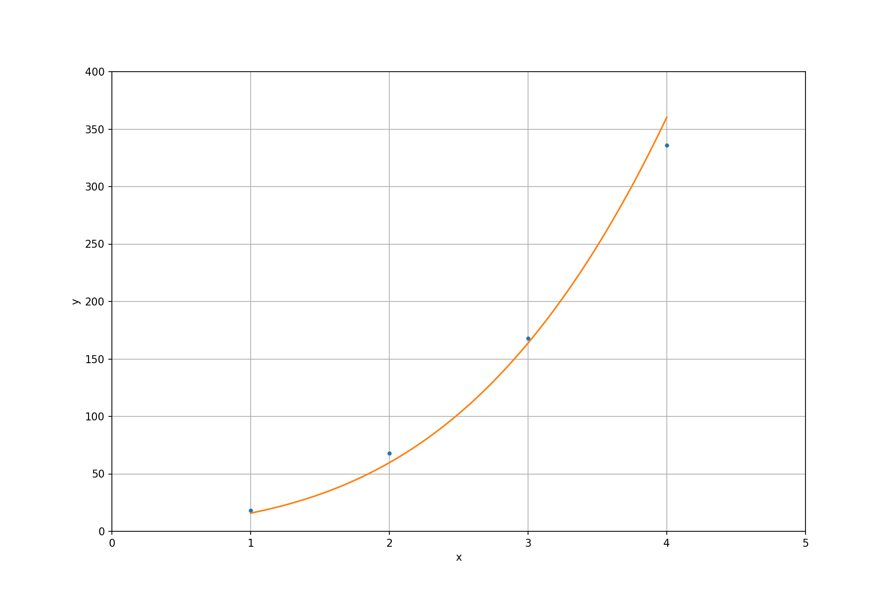
Like the examples of other LAPACK subroutines, we use a simple configuration. Given 4 data points \((1, 17)\), \((2, 58)\), \((3, 165)\), \((4, 360)\). We want to find the closest curve of a polynomial function

\[f(x) = a_1x^3 + a_2x^2 + a_3x\]

The linear system is

\[\begin{split}\mathrm{J} = \left(\begin{array}{ccc} 1 & 1 & 1 \\ 8 & 4 & 2 \\ 27 & 9 & 3 \\ 64 & 16 & 4 \end{array}\right)\end{split}\]

and the right-hand side is

\[\begin{split}\mathbf{y} = \left(\begin{array}{ccc} 17 \\ 58 \\ 165 \\ 360 \end{array}\right)\end{split}\]

Now we can write the code for solving the sample problem:

const size_t m = 4, n = 3;
int status;

std::cout << ">>> least square" << std::endl;
// Use least-square to fit the data of (x, y) tuple:
// (1, 17), (2, 58), (3, 165), (4, 360) to
// the equation: a_1 x^3 + a_2 x^2 + a_3 x.
Matrix mat(m, n, false);
mat(0,0) = 1; mat(0,1) = 1; mat(0,2) = 1;
mat(1,0) = 8; mat(1,1) = 4; mat(1,2) = 2;
mat(2,0) = 27; mat(2,1) = 9; mat(2,2) = 3;
mat(3,0) = 64; mat(3,1) = 16; mat(3,2) = 4;
std::vector<double> y{17, 58, 165, 360};
// The equation f(x) = 3x^3 + 7^2x + 8x can perfectly fit the following
// RHS:
// std::vector<double> y{18, 68, 168, 336};

std::cout << "J:" << mat << std::endl;
std::cout << "y:" << y << std::endl;

status = LAPACKE_dgels(
    LAPACK_ROW_MAJOR // int matrix_layout
  , 'N' // transpose;
        // 'N' is no transpose,
        // 'T' is transpose,
        // 'C' conjugate transpose
  , m // number of rows of matrix
  , n // number of columns of matrix
  , 1 // nrhs; number of columns of RHS
  , mat.data() // a; the 'J' matrix
  , n // lda; leading dimension of matrix
  , y.data() // b; RHS
  , 1 // ldb; leading dimension of RHS
);

std::cout << "dgels status: " << status << std::endl;
std::cout << "a: " << y << std::endl;

The full example code can be found in la05_gels.cpp. The execution results are:

>>> least square
J:
           1          1          1
           8          4          2
          27          9          3
          64         16          4
 data:  1 1 1 8 4 2 27 9 3 64 16 4
y: 17 58 165 360
dgels status: 0
a:  5.35749 -2.04348 12.5266 -2.40772

The last value in a: is garbage and should be ignored. The results tell us the fitted polynomial function is

\[f(x) = 5.35749 x^3 - 2.04348 x^2 + 12.5266 x\]

To make it clearer, we plot the fitted function along with the input points:

Exercises

1. Extend the class Matrix to be an arbitrary dimensional array.

2. Develop your own matrix-matrix multiplication code, measure the runtime, and compare with that of BLAS DGEMM subroutine. The matrix size should be larger than or equal to \(1000\times1000\).

References

[1]

Example Code (Matrix Operations)

[2]

BLAS: http://www.netlib.org/blas/.

[3]

LAPACK: http://www.netlib.org/lapack/.

[4]

MKL: https://software.intel.com/content/www/us/en/develop/tools/oneapi/components/onemkl.html.

[5]

vecLib: https://developer.apple.com/documentation/accelerate/veclib.

[6]

7. Strang, Linear Algebra and Its Applications, 4th ed. Belmont, Calif: Thomson, Brooks/Cole, 2006.

[7]

C11 standard final draft N1570, C 6.7.6.2, April, 2011: http://www.open-std.org/jtc1/sc22/wg14/www/docs/n1570.pdf

[8]

Einstein Summation: https://mathworld.wolfram.com/EinsteinSummation.html

[9]

Strassen, Volker, Gaussian elimination is not optimal, Numer. Math. 13, p. 354-356, 1969. https://doi.org/10.1007/BF02165411